More randomness
Dealing with randomness and random samples of distributions is a huge area, but we're going to finish these posts by considering one last big thing that we haven't touched on at all : random distributions in multiple variables. These look at the question of what happens if you have a set of related variables where the probability of one having a given value of one variable affects the probability of having a given value in another variable. You do have to be a little bit careful though because not all probability functions in more than one variable have this property. A classical example from physics of one that doesn't is the distribution of velocities of particles in a gas.
Particles in a gas are free to move in any direction that they want to, so they have three velocity components since the universe is has 3 spatial dimensions (at least to a good enough approximation for this problem). In fact, the distribution of velocities is given by the Maxwell-Boltzmann distribution, which is basically the Gaussian or Normal distribution that we saw earlier. Mathematically, this looks like

Where Vx, Vy and Vz are the x, y and z components of the particle's velocity, m is the mass of the particle, k is a constant called Boltzmann's constant and T is the temperature in Kelvin (Which is the same as centigrade but offset so that 0C is 273.15K. 0K is "absolute zero" which doesn't exist in nature, so it's fine that this equation breaks at T=0). If you've not seen it before the alpha symbol rather than = means that I'm hiding a constant multiplier in the equation. Using the properties of exponentials we can rewrite this as

Imagine now that you have chosen Vx. That first exponential then just becomes a constant and can be absorbed into the constant that I'm hiding in that alpha symbol so the distribution of Vy and Vz aren't changed by selecting a Vx. That means that I can simply choose Vx, Vy and Vz independently and since they are all Normally distributed I can use the Box-Muller transform that I mentioned in the previous randomness post so I can sample it very fast. Always look at the mathematical description of your distribution to see if you can break it down like this into simpler forms (in more technical language this is termed "seperability" of the equations). It's always faster to sample on a smaller number of variables if at all possible.
But there are some distributions that really can't be separated like this, for example consider

as far as I know this isn't a distribution that anyone is interested in, but it certainly could exist. You can't separate this into functions of Vx, Vy and Vz so you have to sample it in all three variables directly. In the previous post we mentioned inverse transform sampling. This involves forming the cumulative distribution function from the distribution function and sampling along that curve. You can in theory do this for multdimensional functions as well. You have to define a space-filling curve that covers the area of interest of the function and then integrate the PDF along this curve and then finally do inverse sampling along this curve. Doing inverse transform sampling analytically is already tricky and working along an arbitrary curve really doesn't help matters, so in general you have to do it numerically. This means that you have to define your function on a grid of some kind. The problem is that this grid has to have as many dimensions as you have variables, so in this case there's Vx, Vy and Vz so 3D. The more points you have in each dimension of your grid the better your numerical approximation is to the real distribution (you can do things like interpolating between grid points to make it better than the simplest implementation but this is still true overall). So if you want to have 1000 grid points in each direction for this 3D example you'd need between 4 and 8 GB of memory (depending on how you store your numbers, which also affects accuracy). That's possible on a pretty typical computer nowadays, but still a lot of memory. If you had an even harder 4 variable sampling function then this rises to 4-8 TB of memory which is the preserve of high end workstations costing tens of thousands of pounds, and by 6 variable sample functions it couldn't even be run on world leading supercomputers.
Fortunately there is an alternative called rejection sampling. It's much simpler to implement too, although the downside is that it can be much slower to run. You can comparatively easily change any distribution function so that it has a maximum value of 1. Simply find the maximum value in the range of interest of all variables (either analytically or numerically) and divide the distribution function by this value. What you have now is often called the "acceptance function". That is, if I randomly select a value for each variable (selecting this value as a uniform random number in some range of interest), what is the probability that I should accept this value and include it in my sample? This is why the you want a function that has a maximum value of 1 - you want there to be an "optimal" place where acceptance is guaranteed. Then you simply roll one more random value and if it is less than the random probability that you get from the acceptance function then you should take that value, add it to the list of values and continue. If it isn't then you just randomly select new values of all the variablesand keep going until the value is accepted. When you have accepted enough values for your purpose you just stop sampling.
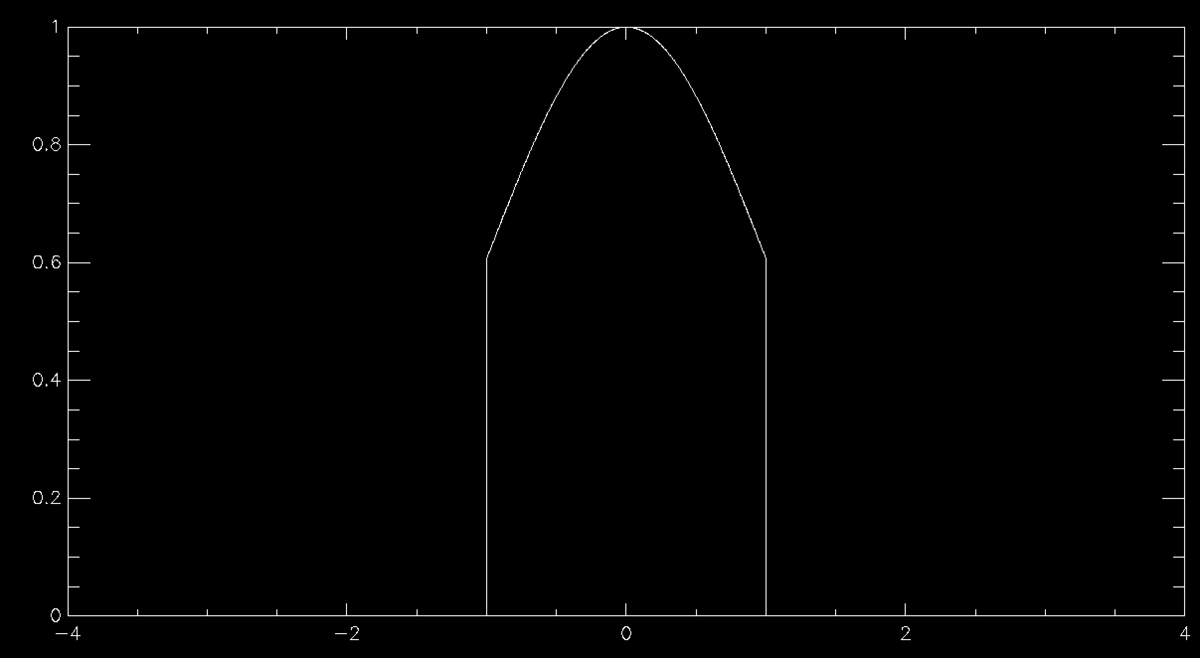
This works beautifully and doesn't require that you allocate any arrays for your distribution function, so long as you can calculate it for any possible value of your variables. Since there's no array there's no problem with discretising the results and you get a nice smooth sample of your distributions function. The problem is in all of the times that you have to throw away sample points because they are rejected. This means that in general rejection sampling is quite slow. While there's no need to, pretend that you want to sample a Normal distribution in a single variable using rejection sampling. If you want to sample it out to one standard deviation from the mean then the average acceptance probability is 86% (ish), so it'll take about 16% longer to compute than it would to be able to simply specify the sample value directly (this isn't quite true because Box-Muller is quite complex and takes longer than a simple rejection sample, but I'm going to ignore this here). Unfortunately there are very few examples of problems where one standard deviation would be enough. In fact, a normal distribution to 1 standard deviation looks quite odd

so you generally have to go further out. At 2 standard deviations you're now accepting about 60% of trials, so you're taking about 66% longer than simple sampling. At 3 standard deviations you're at 42% average acceptance and you're talking about taking 2.4 times longer than a simple sample. At 4 standard deviations you're now down at 31% average acceptance and you've having to do 3 trials for an average sample until you accept it. Unsurprisingly this takes about 3 times longer than simply being able to specify the value, but finally your Normal curve looks about right by eye. As you can see, rejection sampling really should be your last resort since Normal curves are about as benign as distribution functions get - most functions that you'd actually want to run acceptance sampling on have lower acceptance probabilities by the time that you are sampling everything that you want to.
There are more advanced algorithms that are better than rejection sampling (try looking at the Metropolis-Hastings algorithm if you want a place to start), so you're not completely out of luck if you've reached this point and rejection sampling is too slow, but things do start getting more complex from here on in.
 Christopher Brady

 Please wait - comments are loading


 Loading…

