All entries for Thursday 31 May 2018

More randomness and a bit of non–randomness

Normally distributed random numbers

The last blog post was about getting high quality, uniformly distributed random numbers. In this post, I'm going to address the question of what to do if you want to have non uniformly distributed random numbers, that is random numbers where some are more likely than others. One of the ways that we're going to be looking at this is by looking at Probability Distribution Functions(PDF). These graphs are very like histograms, but they instead say "I have a source of random data U. For the entire source U, what is the probability that any given value is in the range x to x + dx, where dx is a finite but usually small deviation from x". In practice, what you do is you split up the range of U into a series of bins of width "dx" and then just count the number of particles in each bin and divide by the total number of particles.

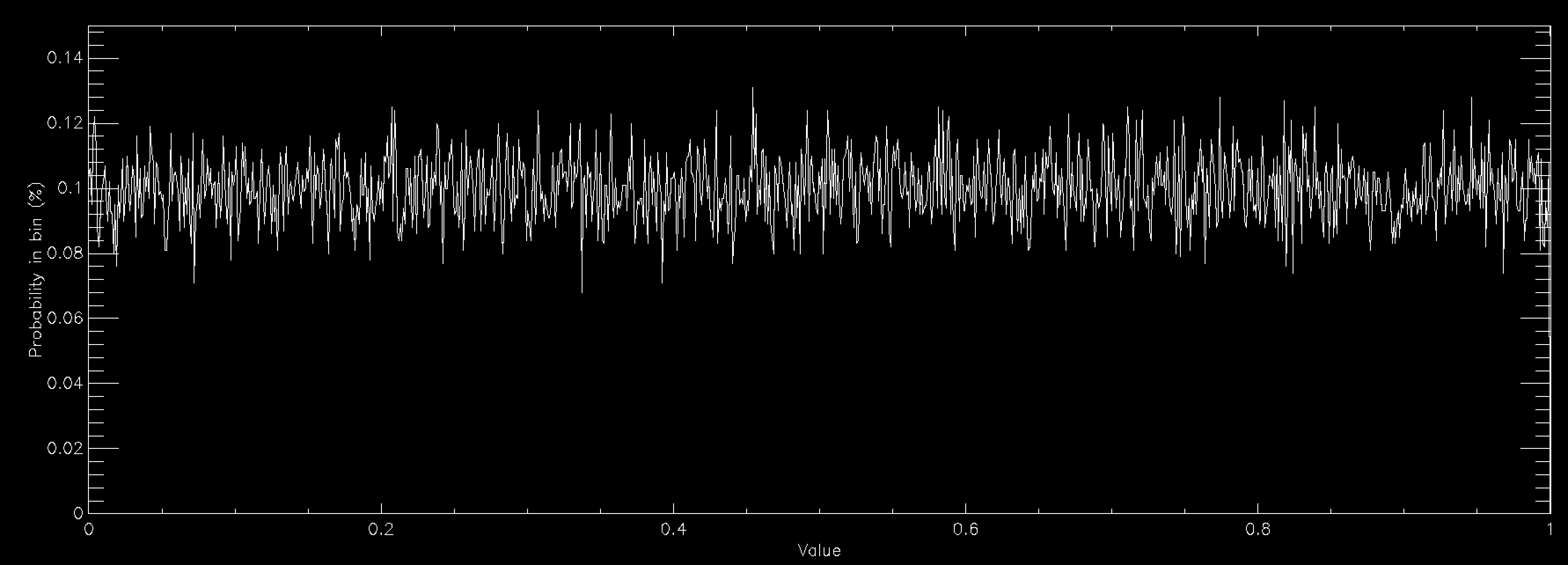
The above graph shows the probability distribution for a uniform random number when you have 1,000 bins between 0 and 1. This number of bins explains why the graph is showing a rough line centred around 0.1% probability. Since a uniform random number generator should produce values in all bins equally, you would expect (100/nbins)% (so 0.1% for 1,000 bins) to lie in each bin. The graph shows that the random number generator that I'm using is working reasonably well.

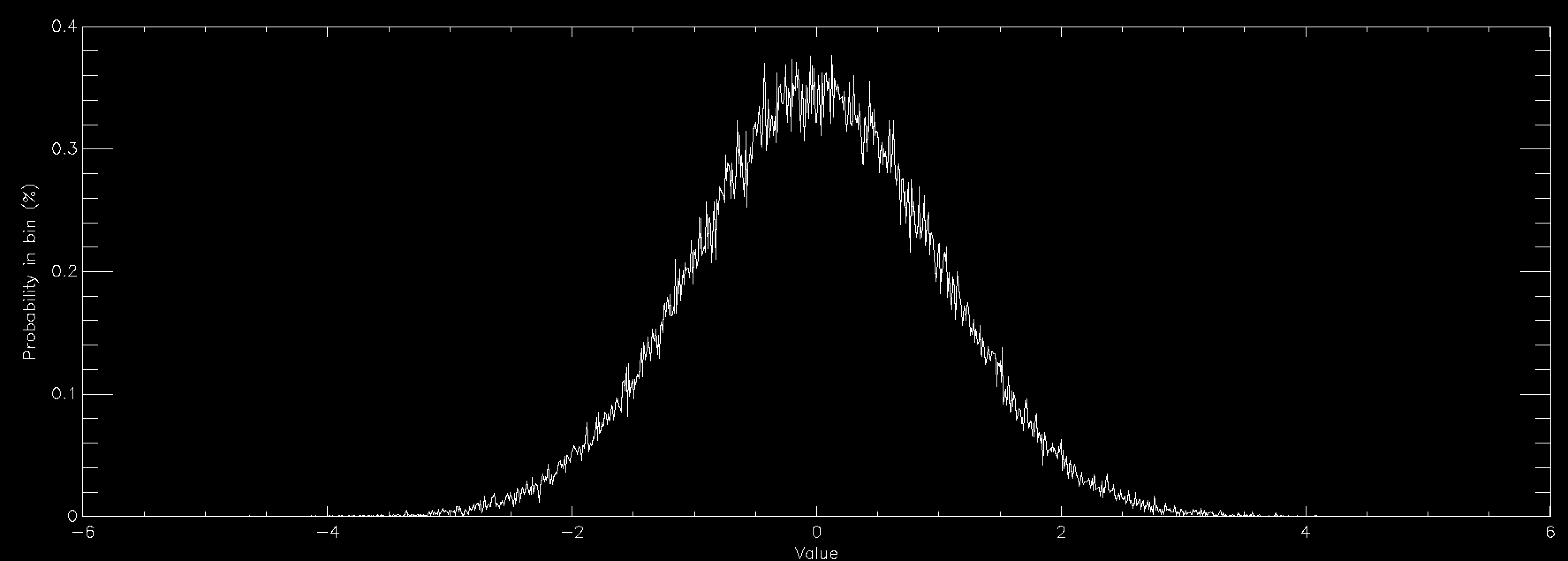
This graph shows the same thing for a normally distributed random number (also called Gaussian, or in some fields Maxwellian distributions and sometimes bell curves). It is strongly peaked at zero and extends out to ±6. Normal distributions are very important in many areas of study (see here for some examples), and is found in things as diverse as the distribution of speeds of particles in a gas to the distribution of heights of members of a sports club. As a consequence there is a lot of interest in generating normally distributed random numbers. This is often called "sampling" the distribution. The graphs above were created by getting random numbers and counting how many fell into each bin on the graph, but often you want to go the other way. You want to draw the graph and then get random numbers such that their distribution will match the graph.

Fortunately there's a very easy way of converting from a uniform random number generator to a normally distributed random number generator via an algorithm called the Box-Muller Transform. I'm not going to go into the maths of it which are detailed on the linked Wikipedia page, but if you want normally distributed random numbers the Box-Muller Transform is your friend (usually the specific variant called the Polar Box-Muller Transform). Lots of languages already have built in implementations of normally distributed random number generators, generally using that transform so it's worth looking for those first, especially in compiled languages like Python where the built in function will probably be much faster than yours. However, in languages like C or Fortran which don't have a built in one you probably want to find or write an implementation of the Box-Muller Transform if you need normally distributed random numbers.

Arbitrary distributions in one variable

Sometimes, however, you have a more complicated distribution function that you want to sample. Sometimes there are other transforms like Box-Muller, but quite often there aren't. At which point the most powerful tool you have is called Inverse Transform Sampling. This introduces a new idea the Cumulative Distribution Function (CDF). The CDF is very much like the PDF in many senses, but instead of saying "how much of U is between x and x+dx" it says "how much of U is between min(U) and x", hence the cumulative in the name. It is the accumulation of the probability of the value being at x or lower.

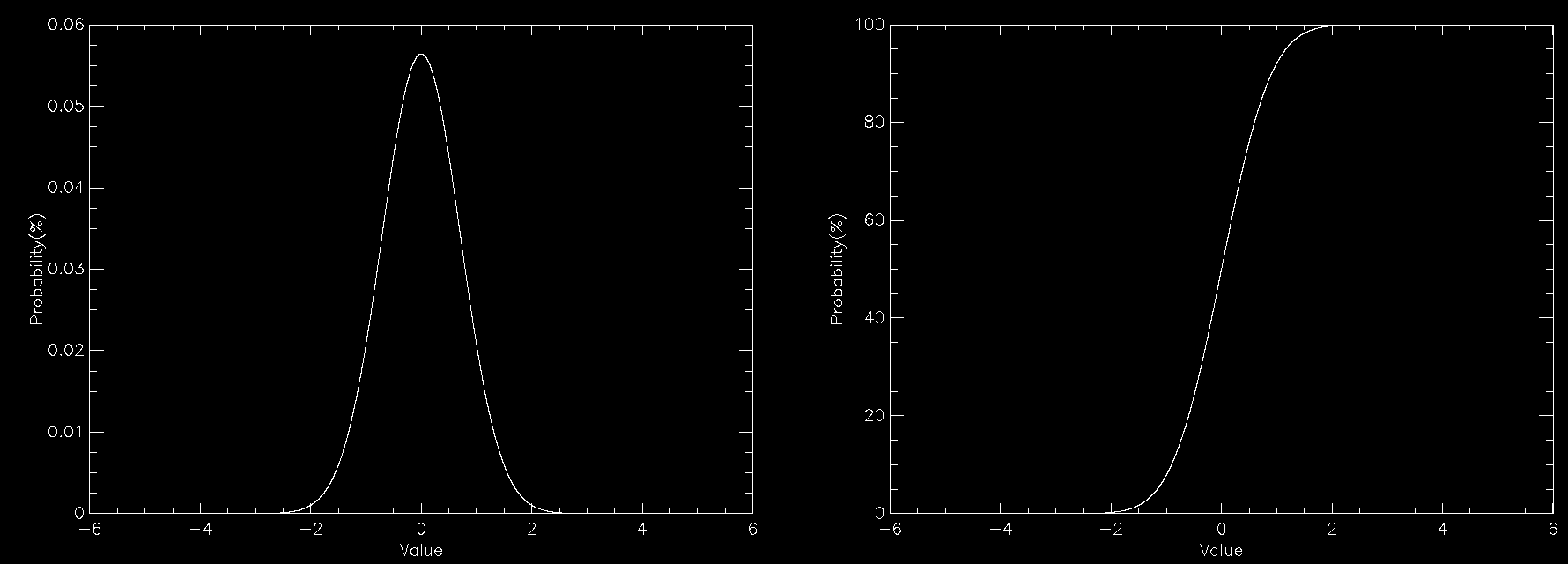
The graph this time compares the PDF (left) to the CDF (right) for a normally distributed number. The CDF has a value of 100% at the right because everything has to be less than the largest value. You can create the CDF in a number of ways, but on a computer a very common way is to define a grid of values (x(i), say) and calculate the PDF (PDF(i)) for each of them. This does mean discretising your distribution but that is often sufficient and you can often interpolate the result. The CDF is then simply defined by

CDF(i) = SUM(PDF(0:i))

where i is the index into a zero based array and is evaluated from 0 to n, where n is the number of elements in the array.

Once you have the CDF sampling it is surprisingly easy. You simply pick a uniform random number between 0 and 100 and then find out which value of i is the cell in which the CDF exceeds that value. You then have sampled the value x(i). You keep repeating this until you have sufficient values. If you then check the distribution of the values it will match the PDF that you specified. Effectively this divides the PDF into bins of equal area under the curve, and selects one bin at a time with equal probability. On the CDF graph, equal area bins correspond to a uniform division of the y axis.

The actual implementation of this can be a bit messier because while the easiest way of finding which cell of the CDF exceeds your random value is simply to start at i=0 and count up, the fastestway is to use binary bisection on the index. This works because the CDF is guaranteed to increase from left to right, so if you pick any point you know if the point that you want is to the left of that point if the value is smaller and to the right of the point if the value is larger. So you can keep dividing the space into sections until you have found the value that you want. But that is an implementation issue rather than a conceptual one.

Note also that if you can integrate the PDF to obtain a CDF, which you can then invert, you can do all of this analytically, but even simple PDFs like a Normal distribution don't have an invertible CDF.

Distributions in more than one variable

Distributions in more than one variable can be tricky. But if the function is separable, that is it can be written as two functions multiplied together, each of which is in a single variable (f(x, y) = g(x) * h(y)) each part can be sampled as above. For each complete sample you take one random sample of the function g, and one of h, and multiply them together.

Functions in more than one variable which don't break down like this are generally treated using a technique called accept-reject sampling, or some more sophisticated technique in tricky cases. More on this next time.

Christopher Brady : 31 May 2018 11:55 |  Tags: Code Programming Randomness |  Comments (0) |  Close comments |  Report a problem