All 22 entries tagged Code

Wherfore art thou – variable names matter!

Sometimes, the simplest questions are the hardest to answer. For instance - what is the meaning of the word "the"? If you've never thought about this, have a go. If you'd prefer a non-grammar, or non-English specific example, try to describe the number '1'. Trickier than you'd think, isn't it?

But that is hardly relevant to programming, so lets look at today's deceptively simple question instead. Namely, how long should variable and function names be?

Some people might seem to have an answer to this question, such as "between one and five words, usually two or more". They are wrong. Any answer containing numbers is unhelpful and either sometimes wrong, or too broad to mean anything. For instance, "Supercalifragilisticexpialidocious" [typed from memory... excuse spelling] is one word, and is terrible. And "SolveWaveEquationSecondOrderWithLimiter" is seven and (in the right context) is quite good. "FlagSettingWhetherWeShouldPrintTheAnswerToScreenOrNot" is clearly terrible - but it is thoroughly descriptive.

So why do we struggle so much to answer this question? Because we are in a sort of "tug-of-war" between two competing interests, and which one pulls a little harder depends on a lot of things. Both ends of the rope are anchored in clarity: on the one hand we want maximum clarity for the function - a very descriptive name. This tends to favour longer names, with more detail. On the other hand, we want maximum clarity for the code as a whole - a name that doesn't take up too much mental space in a block of code. This tends to favour shorter names, with fewer, simpler words. To find our optimum, we must somehow balance these two.

A brief aside here into our absolute best weapon in this - make the two ends stop pulling. Find a way to make "descriptive" and "compact" the same thing. Specialised definitions of terms specific to a field of interest, i.e. jargon, really works in our favour here. We must use it with caution, because new jargon can be very jarring and difficult to master, but in general jargon terms are addressing exactly the same problem - descriptive yet compact terms. For instance, a word you may barely think of as jargon - "laptop". Let us expand this definition - perhaps we get "a portable, all-in-one computing device". But we still have some specialised terms here - what is "all-in-one"? What is "computing"? We could continue the expansion almost indefinitely. Or, we can simply use the term "laptop" and in most cases be perfectly understood.

It is important to flag here that word, "most". Is a tablet a laptop? If I strap a monitor to a tower PC and plug in a keyboard, do I have a "laptop"? It's going to depend on context whether those are reasonable (OK, the second one is extremely unlikely to be). But consider similar questions - "do you have a car?" "No, I have a van" - sensible answer, or irritating pedant? "We need to seat 5 people, who has a car?" "I have an MX5" - as it turns out, "car" doesn't always mean 5 seats.

Back from our aside now, new weapon in hand. Careful, selective use of jargon can make our names very descriptive, while remaining compact. If the jargon we use is not universal, we can provide a glossary or add context in our docs. We should be very very careful about making up our own jargon here, because unfamiliar terms can lead to misunderstanding, but if your field provides words, exploit them.

One last important point - sometimes an otherwise optimal name is not useful due to ambiguity. This can be typographical - we should never have names that differ only in characters like '1' and 'l' or differ only in the case (small or CAPITAL) of the letters. Ambiguity can be similarity with some other function name - imagine we somehow tried to have "GetDiscreteName" and "GetDiscreetName" - could you even tell those apart? Ambiguity is an enemy of clarity - avoid it.

OK, actually there is one final point. Clearly redundancy can only harm our compactness of names. But it does have some applications. We might want two functions with very similar names, but different parameters - "SolveTypeAEquation(a, b, c)" and "SolveTypeAEquationNormalised(a, b, param)" for instance. If we can't design the code to make these less confusing, we might deliberately make one name less individually clear, if it makes its usage clearer. So perhaps the second one becomes "SolveTypeAEquationNormalisedWithParam(a, b, param)" which repeats information already in the signature (redundancy), but helps us keep in mind which function we want.

Short posts like this rarely have conclusions, because everything has already been said, usually repeatedly. Since repetition is another form of redundancy that actually works though, lets restate our key point:

We must balance the demands of clarity between our functions and our wider code and try and find a name which is BOTH descriptive and also short and easy to handle. Sometimes one of these will be a bit more important, sometimes the other.

Heather Ratcliffe : 06 Jun 2022 13:41 |  Tags: Code Philosophy Programming Shortpost |  Comments (0) |  Close comments |  Report a problem

License choice in the R community

This week a post on the RSE Slacksparked a lot of discussion on how to choose a license for your research software. The website https://choosealicense.com/is a helpful resource and starts with an important point raised by Hugo Grusonthat a good place to start is to consider the license(s) commonly used in your community. But how do you find out this information? This blog post explores the licenses used in the R and Bioconductor communities, by demonstrating how to obtain licencing information on CRAN and Bioconductor packages.

Licenses on CRAN

The Comprehensive R Archive Network (CRAN) repository is the main repository for R packages and the default repository used when installing add-on packages in R. The tools package that comes with the base distribution of R provides the CRAN_package_db() function to download a data frame of metadata on CRAN packages. Using this function, we can see that there are currently 19051 packages on CRAN.

library(tools)
pkgs <- CRAN_package_db()
nrow(pkgs)

## [1] 19051

The license information is in the License column of the data frame. We'll use the dplyr package to help summarise this variable. With n_distinct() we find that there are 164 unique licenses!

library(dplyr)
n_distinct(pkgs$License)

## [1] 164

However, many of these are different versions of a license, e.g.

pkgs |>
  filter(grepl("^MIT", License)) |>
  distinct(License)

##                                   License
## 1                      MIT + file LICENSE
## 2              MIT License + file LICENSE
## 3                      MIT + file LICENCE
## 4 MIT + file LICENSE | Apache License 2.0
## 5                       MIT +file LICENSE
## 6          MIT + file LICENSE | Unlimited

The above output also illustrates that

• An additional LICENSE (or LICENCE) file can be used to add additional terms to the license (the year and copyright holder in the case of MIT).
• Packages can have more than one license (the user can choose any of the alternatives).
• Authors do not always provide the license in a standard form!

A LICENSE file can also be used to on its own to specify a non-standard license. Given this variation in license specification, we will use transmute() to create a new set of variables, counting the number of times each type of license appears in the specification. We create a helper function n_match() to count the number of matches for a regular expression, which helps to deal with variations in the form provided. Finally we check against the expected number of licenses for each package to check we have covered all the options.

n_match <- function(s, x) lengths(regmatches(x, gregexpr(s, x)))
licenses <- pkgs |>
  transmute(
    ACM = n_match("ACM", License),
    AGPL = n_match("(Affero General Public License)|(AGPL)", License),
    Apache = n_match("Apache", License),
    Artistic = n_match("Artistic", License),
    BSD = n_match("(^|[^e])BSD", License),
    BSL = n_match("BSL", License),
    CC0 = n_match("CC0", License),
    `CC BY` = n_match("(Creative Commons)|(CC BY)", License),
    CeCILL = n_match("CeCILL", License),
    CPL = n_match("(Common Public License)|(CPL)", License),
    EPL = n_match("EPL", License),
    EUPL = n_match("EUPL", License),
    FreeBSD = n_match("FreeBSD", License),
    GPL = n_match("((^|[^ro] )General Public License|(^|[^LA])GPL)", License),
    LGPL = n_match("(Lesser General Public License)|(LGPL)", License),
    LICENSE = n_match("(^|[|] *)file LICEN[SC]E", License),
    LPL = n_match("(Lucent Public License)", License),
    MIT = n_match("MIT", License),
    MPL = n_match("(Mozilla Public License)|(MPL)", License),
    Unlimited = n_match("Unlimited", License))
n_license <- n_match("[|]", pkgs$License) + 1
all(rowSums(licenses) == n_license)

## TRUE

Now we can tally the counts for each license, discounting version differences (i.e., GPL-2 | GPL-3 would only count once for GPL). We convert the license variable into a factor so that we can order by descending frequency in a plot.

tally <- colSums(licenses > 0)
tally_data <- 
  tibble(license = names(tally),
         count = tally) |>
  arrange(desc(count)) |>
  mutate(license = factor(license, levels = license))

tally_data.csv

The vast majority are GPL (73%), followed by MIT (18%). All other licenses are represented in less than 3% of packages. This is consistent with R itself being licensed under GPL-2 | GPL-3. The only licenses in the top 10 that are not mentioned as "in use" on https://www.r-project.org/Licenses/, are the Apache and CC0 licenses, used by 1.7% and 1.1% of packages, respectively. The Apache license is a modern permissive license similar to MIT or the older BSD license, while CC0 is often use for data packages where attribution is not required. A separate LICENSE file is the 3rd most common license among CRAN packages; without exploring further it is unclear if this is always a stand-alone alternative license (as the specification implies) or if it might sometimes be adding further terms to another license.

Licenses on Bioconductor

Bioconductor is the second largest repository of R packages (excluding GitHub, which acts as a more informal repository). Bioconductor specialises in packages for bioinformatics. We can conduct a similar analysis to that for CRAN using the BiocPkgToolspackage. The function to obtain metadata on Bioconductor packages is biocPkgList(). With this we find there are currently 2041 packages on Bioconductor:

library(BiocPkgTools)
pkgs <- biocPkgList()
nrow(pkgs)

## [1] 2041

Still, there are 89 distinct licenses among these pckages:

n_distinct(pkgs$License)

## [1] 89

We can use the same code as before to tally each license and create a plot - the only change made to create the plot below was to exclude licenses that were not represented on Bioconductor.

tally_data_bioc.csv

GPL is still a popular license, represented by 55% of packages. However the Artistic license is also popular in this community (23%). This reflects the fact that the Bioconductor core packages are typically licensed under Artistic-2.0 and community members may follow the lead of the core team. Third to fifth place are taken by MIT (9%), LGPL (7%) and LICENSE (4%), respectively, with the remaining licenses represented in less than 2% of packages. The ACM, BSL, CC0, EUPL, FreeBSD and LPL licenses are unrepresented here.

Summary

Although the Biconductor community is a subset of the R community, it has different norms regarding package licenses. In both communities though, the GPL is a common choice for licensing R packages, consistent with the license choice for R itself.

Heather Turner : 08 Apr 2022 10:32 |  Tags: Code Licenses R |  Comments (0) |  Close comments |  Report a problem

What's the time right now?

This is not one of my mistakes, this is one I read about second hand (you'll see the pun in a moment), but it is a great illustration of the importance of writing the code you actually mean to, thinking properly about what it is that you mean, and watching out for weasel words that might confuse you.

Consider these two lines of code and decide for youself whether they have the same effect:

if (DateTime.Now.Second == 0 && DateTime.Now.Minute == 0)

if (DateTime.Now.Minute == 0 && DateTime.Now.Second == 0)

Decided yet? If you think they are the same, take a second now (that's a hint!) to think about the meaning of each part, and what its value will be. Suppose the original author intended to run some process once per hour, so put one of these into a loop. Can you see why one of these might succeed, and the other fail occasionally (assume the rest of the code takes some tiny fraction of a second)?

By the way, if you're worried about not knowing what language this is in, don't be. This is a perfect example of good "self documenting code" which we've written a bit about before. Based on the names, we can infer (correctly) that DateTime is some sort of thing, which can supply the date-and-time Now through the "DateTime.Now" construct, and that we can then look at the Minutes and Seconds value of the time Now. That's all we need to know.

So, back to the question. Are the lines the same? Well, the order is different. There's a double-& AND operation. We don't strictly know whether the left or right condition will be checked first (it might depend on language), and we don't actually know if both will be (if you're not sure why that is, we've talked about short circuiting in logical operations here). But that shouldn't matter unless the DateTime object is having some weird side-effects and I promise it isn't. The problem is much more fundamental than that.

If you haven't spotted it, it's time to write down very clearly what we wanted to check. We want to know if, right now, the value of both the minutes and the seconds entries are 0. It looks like that's what either line does, but there's a nasty weasly word sneaking in here - the word "now". What can "now" actually mean in programming terms, where we know operations ultimately are carried out one by one in sequence? For instance, what would you expect the following code could print?

if (DateTime.Now.Second == 0) print(DateTime.Now.Second)


If you said 0 only, hold on a second (that's a hint, too) and look again, and think about what this code will actually do in terms of basic operations. It will get a value for DateTime.Now.Second. It will compare this to 0. If the comparison is true it will get a value for DateTime.Now.Second, and it will print this value. And there is the problem! The value we check and the value we print are not always the same.

If it still isn't clear to you why the original two lines are not equivalent, reread that last paragraph a few times and apply the same idea to the original question. If it's been obvious to you all along, great. You're unlikely to make the mistake this original programmer did. But why did they make this mistake? There could be several reasons:

• They might simply not have spotted there could be a problem - this is pretty likely, but not very interesting
  
• They might have thought somehow the compiler/runtime would recognise the values as "the same" - this is a pretty fundamental mistake, perhaps due to thinking of "Now" as a property rather than an operation. In some very imprecise sense, we should think of "Now" as having a side-effect on itself because it takes time, so multiple calls will not have the same result as a single one
  
• They might have blindly removed a temporary variable containing DateTime.Now, without thinking deeply about the consequences. This is quite likely because it looks so simple, and is why refactoring like this needs, if anything, more attention than writing the code in the first place
  
• Lastly, they might have thought carefully and precisely, but ultimately wrongly about it. If they confused the idea of seconds as a time point with seconds as a time interval, they may have thought that both the Seconds and the Minutes property would surely be evaluated within the same second, and thus work as expected, where actually even a microsecond between them could be the difference between 1:59.999 and 2:00.000
  

So, that explains why the lines don't work as intended, but there's one weird thing left - how come one of them (the first one, if evaluation occurs left to right) works, but the other doesn't? Effectively, the minutes value depends on the seconds value - the minute is incremented only when the seconds reads 59. We know the whole operation takes far far less than 1 second (ignoring interrupts or anything else suspending operation), so once we have confirmed the seconds value as 0, we have at least 59-60 seconds to check the minutes value, during which it cannot change. Certainly this will occur within that interval, and the code will work perfectly (again, ignoring external iterrupts, which our code can never account for anyway).

So, does that mean the first option is actually safe, or good code? Well, not without a comment it certainly isn't! If we're relying on this sort of subtlety, somebody is going to be tripped up by it, and it might even be us. It's also a bit delicate - suppose we were to need to use DateTime.Now in another part of the condition, or in the body? We'd have to think very hard about whether we're still "safe" and we simply don't need to. A temporary variable is much clearer, and the possible optimisation here is a) tiny and b) best left to our compiler anyway. Oh and c) possibly a de-optimisation anyway, depending on the cost of the DateTime.Now lookup. Also, it'd be easy to forget that the left-to-right ordering is important, and we might try this in a situation or language where that is not guaranteed.

Ultimately, I simply don't like relying on such a subtlety. It's too clever and it doesn't need to be. It's not that I don't like clever code, because I do. I like clever code that makes one exclaim "oh yes, that's so simple, it's brilliant", and this aint that. This is more "oh blimey, is that how it works". Keep it simple, and if you can't keep it simple, at least make it satisfying.

Postscript

Before we go, I hope something has been nagging at you throughout this post. I started off by saying we should think hard about what we mean and what we want to actually do. I introduced this idea of minute-0 and second-0 and then proposed it as a solution to doing something once per hour. Did it strike you as a pretty terrible solution to that problem? Because it is. Suppose we start running our code at 9:00:30 AM. Would we expect whatever this block controls to wait an entire hour to fire for the first time? What if the code is never running at the change of the hour? This block would never run. Suppose we start 1000 copies of this code. Do we really want all 1000 to execute this block at the same time? Suppose some other code took longer than expected and this block isn't reached once per second - some hours might be simply skipped. In nearly all cases we'd be better checking whether at least an hour has elapsed since last we did the thing, and we'd avoid all of these problems. We meant once per hour, not on the first second of every hour, and we should have coded that, not this.

This post is inspired by an article I read a while ago, namely https://thedailywtf.com/articles/an-hourly-rate In particular, a comment mentions the different behaviour of the two possible lines, which this post focuses on.

Heather Ratcliffe : 07 Mar 2022 16:11 |  Tags: Bugs Code Programming |  Comments (0) |  Close comments |  Report a problem

Learning to Program

We (Warwick RSE) love quotes, and we love analogies. We do always caution against letting your analogies leak, by supposing properties of the model will necessarily apply to reality, but nontheless, a carefully chosen story can illustrate a concept like nothing else. This post discusses some of my favorite analogies for the process of learning to program - which lasts one's entire programming life, by the way. We're never done learning.

Jigsaw Puzzles

Learning to program is a lot like trying to complete a jigsaw puzzle without the picture on the box. At first, you have a blank table and a heap of pieces. Perhaps some of the pieces have snippets you can understand already - writing perhaps, or small pictures. You know what these depict, but not where they might fit overall. You start by gathering pieces that somehow fit together - edges perhaps, or writing, or small amounts of distinctive colours. You build up little blocks (build understanding of isolated concepts) and start to fit them together. As the picture builds up, new pieces fit in far more easily - you use the existing picture to help you understand what they mean. Of course, the programming puzzle is never finished, which is where this analogy starts to leak.

I particularly like this one for two reasons. Firstly, one really does tend to build little isolated mini-pictures, and move them around the table until they start to connect together, both in jigsaws and in programming. Secondly, occasionally, you have these little moments - a piece that seemed to be just some weird lines fits into place and you say "oh is THAT what that is!". One gets the same thing when programming - "oh, is that how that works!" or "is that what that means".

Personally, a lot of these moments then become "Why didn't anybody SAY that!". This was the motivation behind our blog series of "Well I Never Knew That" - all those little things that make so much sense once you know.

The other motivation for the WINKT series is better illustrated using a different analogy - hence why we like to have plenty on hand.

A Walk in the Woods

Another way to look at the learning process, is as a process of exploring some new terrain, building your mental map of it. At first, you mostly stick to obvious paths, slowly venturing further and further. You find landmarks and add them to your map. Some paths turn out to link up to other paths, and you start to assemble a true connected picture of how things fit together. Yet still there is terrain just off the paths you haven't gone into. There could be anything out there, just outside your view. Even as you venture further and deeper into the woods, you must also make sure to look around you, and truly understand the areas you've already walked through, and how they connect together.

My badly done keynote picture is below. The paths are thin lines, the red fuzzy marks show those we have explored and the grey shading shows the areas we've actually been into and now "understand". Eventually we notice that the two paths in the middle are joined - a nice "Aha" moment of clarity ensues. But much of our map remains a mystery.

And that is one of the reasons I really like this analogy - all of the things you still don't know - all that unexplored terrain. This too is very like the learning process - you are able to use things once you have walked their paths, even though there may be details about them you don't understand. On the one hand, this is very powerful. On the other, it can lead to "magic incantations" - things you can repeat without actually understanding. This is inevitable in a task this complex, but it is important to go back and understand eventually. Don't let your map get too thin and don't always stick to the paths, or when you do step off them, you'll be lost.

This was the other main motivation behind our WINKT series - the moments when things you do without thinking suddenly make sense, and a new chunk of terrain gets filled in. Like approaching the same bit of terrain from a new angle, or discovering that two paths join, you gain a new perspective, and ideally, this new perspective is simpler than before. Rather than two paths, you see there is only one. Rather than two mysterious houses deep in the woods, you see there is one, seen from two angles.

Take Away Point

If you take one thing away from this post, make it this: the more you work on fitting the puzzle pieces together, the clearer things become. Rather than brown and green and blue and a pile of mysterious shapes, eventually you just have a horse.

And one final thing, if we may stretch the jigsaw analogy a little further: just because a piece seems to fit, doesn't mean it's always the right piece...

Heather Ratcliffe : 02 Mar 2022 12:52 |  Tags: Code Philosophy Programming Winkt |  Comments (0) |  Close comments |  Report a problem

Advent of Code 2021: First days with R

The Advent of Code is a series of daily programming puzzles running up to Christmas. On 3 December, the Warwick R User Group met jointly with the Manchester R-thritis Statistical Computing Group to informally discuss our solutions to the puzzles from the first two days. Some of the participants shared their solutions in advance as shared in this slide deck.

In this post, Heather Turner (RSE Fellow, Statistics) shares her solutions and how they can be improved based on the ideas put forward at the meetup by David Selby (Manchester R-thritis organizer) and others, while James Tripp (Senior Research Software Engineer, Information and Digital Group) reflects on some issues raised in the meetup discussion.

R Solutions for Days 1 and 2

Heather Turner

Day 1: Sonar Sweep

For a full description of the problem for Day 1, see https://adventofcode.com/2021/day/1.

Day 1 - Part 1

How many measurements are larger than the previous measurement?

199  (N/A - no previous measurement)
200  (increased)
208  (increased)
210  (increased)
200  (decreased)
207  (increased)
240  (increased)
269  (increased)
260  (decreased)
263  (increased)

First create a vector with the example data:

x <- c(199, 200, 208, 210, 200, 207, 240, 269, 260, 263)

Then the puzzle can be solved with the following R function, that takes the vector x as input, uses diff() to compute differences between consecutive values of x, then sums the differences that are positive:

f01a <- function(x) {
  dx <- diff(x)
  sum(sign(dx) == 1)
}
f01a(x)

## [1] 7

Inspired by David Selby’s solution, this could be made slightly simpler by finding the positive differences with dx > 0, rather than using the sign() function.

Day 1 - Part 2

How many sliding three-measurement sums are larger than the previous sum?

199  A           607  (N/A - no previous sum)
200  A B         618  (increased)
208  A B C       618  (no change)
210    B C D     617  (decreased)
200  E   C D     647  (increased)
207  E F   D     716  (increased)
240  E F G       769  (increased)
269    F G H     792  (increased)
260      G H
263        H

This can be solved by the following function of x. First, the rolling sums of three consecutive values are computed in a vectorized computation, i.e. creating three vectors containing the first, second and third value in the sum, then adding the vectors together. Then, the function from Part 1 is used to sum the positive differences between these values.

f01b <- function(x) {
  n <- length(x)
  sum3 <- x[1:(n - 2)] + x[2:(n - 1)] + x[3:n]
  f01a(sum3)
}
f01b(x)

## [1] 5

David Schoch put forward a solution that takes advantage of the fact that the difference between consecutive rolling sums of three values is just the difference between values three places apart (the second and third values in the first sum cancel out the first and second values in the second sum). Putting what we’ve learnt together gives this much neater solution for Day 1 Part 2:

f01b_revised <- function(x) {
  dx3 <- diff(x, lag = 3)
  sum(dx3 > 0)
}
f01b_revised(x)

## [1] 5

Day 2: Dive!

For a full description of the problem see https://adventofcode.com/2021/day/2.

Day 2 - Part 1

• forward X increases the horizontal position by X units.
• down X increases the depth by X units.
• up X decreases the depth by X units.

                  horizontal  depth
forward 5   -->            5      -
down 5      -->                   5
forward 8   -->           13
up 3        -->                   2
down 8      -->                  10
forward 2   -->           15

==> horizontal = 15, depth = 10

First create a data frame with the example data

x <- data.frame(direction = c("forward", "down", "forward",
                              "up", "down", "forward"),
                amount = c(5, 5, 8, 3, 8, 2))

Then the puzzle can be solved with the following function, which takes the variables direction and amount as input. The horizontal position is the sum of the amounts where the direction is “forward”. The depth is the sum of the amounts where direction is “down” minus the sum of the amounts where direction is “up”.

f02a <- function(direction, amount) {
  horizontal <- sum(amount[direction == "forward"])
  depth <- sum(amount[direction == "down"]) - sum(amount[direction == "up"])
  c(horizontal = horizontal, depth = depth)
}
f02a(x$direction, x$amount)

## horizontal      depth 
##         15         10

The code above uses logical indexing to select the amounts that contribute to each sum. An alternative approach from David Selby is to coerce the logical indices to numeric (coercing TRUE to 1 and FALSE to 0) and multiply the amount by the resulting vectors as required:

f02a_selby <- function(direction, amount) {
  horizontal_move <- amount * (direction == 'forward')
  depth_move <- amount * ((direction == 'down') - (direction == 'up'))
  c(horizontal = sum(horizontal_move), depth = sum(depth_move))
}

Benchmarking on 1000 datasets of 1000 rows this alternative solution is only marginally faster (an average run-time of 31 μs vs 37 μs), but it has an advantage in Part 2!

Day 2 - Part 2

• down X increases your aim by X units.
• up X decreases your aim by X units.
• forward X does two things:
  • It increases your horizontal position by X units.
  • It increases your depth by your aim multiplied by X.

                  horizontal  aim  depth
forward 5   -->            5    -      - 
down 5      -->                 5      
forward 8   -->           13          40
up 3        -->                 2
down 8      -->                10
forward 2   -->           15          60

==> horizontal = 15, depth = 60

The following function solves this problem by first computing the sign of the change to aim, which is negative if the direction is “up” and positive otherwise. Then for each change in position, if the direction is “forward” the function adds the amount to the horizontal position and the amount multiplied by aim to the depth, otherwise it adds the sign multiplied by the amount to the aim.

f02b <- function(direction, amount) {
  horizontal <- depth <- aim <- 0
  sign <- ifelse(direction == "up", -1, 1)
  for (i in seq_along(direction)){
    if (direction[i] == "forward"){
      horizontal <- horizontal + amount[i]
      depth <- depth + aim * amount[i]
      next
    }
    aim <- aim + sign[i]*amount[i]
  }
  c(horizontal = horizontal, depth = depth)
}
f02b(x$direction, x$amount)

## horizontal      depth 
##         15         60

As an interpreted language, for loops can be slow in R and vectorized solutions are often preferable if memory is not an issue. David Selby showed that his solution from Part 1 can be extended to solve the problem in Part 2, by using cumulative sums of the value that represented depth in Part 1 to compute the aim value in Part 2.

f02b_revised <- function(direction, amount) {
  horizontal_move <- amount * (direction == "forward")
  aim <- cumsum(amount * (direction == "down") - amount * (direction == "up"))
  depth_move <- aim * horizontal_move
  c(horizontal = sum(horizontal_move), depth = sum(depth_move))
}
f02b_revised(x$direction, x$amount)

## horizontal      depth 
##         15         60

Benchmarking these two solutions on 1000 data sets of 1000 rows, the vectorized solution is ten times faster (on average 58 μs vs 514 μs).

Reflections

James Tripp

How do we solve a problem with code? Writing an answer requires what some educators call computational thinking. We systematically conceptualise the solution to a problem and then work through a series of steps, drawing on coding conventions, to formulate an answer. Each answer is different and, often, a reflection of our priorities, experience, and domains of work. In our meeting, it was wonderful to see people with a wide range of experience and differing interests.

Our discussion considered the criteria of a ‘good solution’.

• Speed is one criteria of success - a solution which takes 100 μs (microseconds) is better than a solution taking 150 μs.
• Readability for both sharing with others (as done above) and to help future you, lest you forget the intricacies of your own solution.
• Good practice such as variable naming and, perhaps, avoiding for loops where possible. Loops are slower and somewhat discouraged in the R community. However, some would argue they are more explicit and helpful for those coming from other languages, such as Python.
• Debugging friendly.Some participants, including Heather Turner and David Selby, checked their solutions with tests comparing known inputs and outputs. I drew on my Psychology experience and opted for an explicit DataFrame where I can see each operation. Testing is almost certainly a better solution which I adopt in my packages.
• Generalisability. A solution tailored for the Part 1 task on a given day may not be easily generalisable for the Part 2 task. It seemed desirable to refactor one’s code to create a solution which encompasses both tasks. However, the effort and benefits of doing so are certainly debatable.

We also discussed levels of abstraction. The tidyverse family of R packages is powerful, high-level and quite opinionated. Using tidyverse functions returned some intuitive, but slower solutions where we were unsure of the bottlenecks. Solutions built on R base (the functions which come with R) were somewhat faster, though others using libraries such as data.table were also rather quick. These reflections are certainly generalisations and prompted some discussion.

How does one produce fast, readable, debuggable, generalisable code which follows good practice and operates at a suitable level of abstraction? Our discussions did not produce a definitive answer. Instead, our discussions and sharing solutions helped us understand the pros and cons of different approaches and I certainly learned a few useful tricks.

Heather Turner : 08 Dec 2021 10:00 |  Tags: Code Programming R |  Comments (0) |  Close comments |  Report a problem

Scheduling of OpenMP

OpenMP is one of the most popular methods in academic programming to write parallel code. It's major advantage is that you can achieve performance improvements in a lot of cases by just putting "directives" into your code to tell the compiler "You can take this loop and split it up into sections for each processor". Other parallelism schemes like MPI or Intel Threaded Building Blocks or Coarray Fortran all involve designing your algorithm around splitting the work up, OpenMP makes it easy to simply add parallelism to bits where you want it. (There are also lots of bits of OpenMP programming that require you to make changes to your code but you can get further than in pretty much any other modern paradigm without having to alter your actual code).

So what does this look like in practice?

 
MODULE prime_finder
  USE ISO_FORTRAN_ENV
  IMPLICIT NONE

  INTEGER(INT64), PARAMETER ::  small_primes_len = 20
  INTEGER(INT64), DIMENSION(small_primes_len), PARAMETER :: &
      small_primes = [2, 3, 5, 7, 11, 13, 17, 19, 23, 29, 31, 37, 41, 43, 47, &
      53, 59, 61, 67, 71]
  INTEGER, PARAMETER :: max_small_prime = 71

  CONTAINS

  FUNCTION check_prime(num)
    INTEGER(INT64), INTENT(IN) :: num
    LOGICAL :: check_prime

    INTEGER(INT64) :: index, end

    end = CEILING(SQRT(REAL(num, REAL64)))

    check_prime = .FALSE.
    !First check against the small primes
    DO index = 1, small_primes_len
      IF (small_primes(index) == num) THEN
        check_prime = .TRUE.
        RETURN
      END IF
      IF (MOD(num, small_primes(index)) == 0) THEN
        RETURN
      END IF
    END DO

    !Test higher numbers, skipping all the evens
    DO index = max_small_prime + 2, end, 2
      IF (MOD(num, index) == 0) RETURN
    END DO
    check_prime = .TRUE.
  END FUNCTION check_prime

END MODULE prime_finder

PROGRAM primes

  USE prime_finder
  IMPLICIT NONE
  INTEGER(INT64) :: ct, i

  ct = 0_INT64
!$OMP PARALLEL DO REDUCTION(+:ct)
  DO i = 2_INT64, 20000000_INT64
    IF (check_prime(i)) ct = ct + 1
  END DO
!$OMP END PARALLEL DO

  PRINT *, "Number of primes = ", ct

END PROGRAM primes

This is a Fortran 2008 program (although OpenMP works on Fortran, C and C++) that uses a very simple algorithm to count the number of prime numbers between 2 and 20,000,000. There are much better algorithms for this but this algorithm correctly counts this number of primes and is very suitable for parallelising since each number is checked for primality separately. This code is already OpenMP parallelised and as you can see the parallelism is very simple. The only lines of OpenMP code are !$OMP PARALLEL DO REDUCTION(+:ct)and$OMP END PARALLEL DO . The first line says that I want this loop to be parallel and that the variable ct should be calculated separately on each processor and then summed over all processors at the end. The second line just says that we have finished with parallelism and should switch back to running the code in serial after this point. Otherwise that is exactly the same program that I would have written if I was testing the problem on a single processor and I get the result that there are 1,270,607 primes less than 20,000,000 regardless of how many processors I run on. So far so good but look what happens when I look at the timings for different numbers of processors

Number of Processors	Time(s)
1	11.3
2	7.2
4	3.9
8	2.2
16	1.13

It certainly speeds up! But not as much as it should since every single prime is being tested separately (the number for 16 processors would be 0.71 seconds if it was scaling perfectly). There are lots of reasons why parallel codes don't speed up as much as they should but in this case it isn't any underlying limitation of the hardware but is to do with how OpenMP chooses to split up my problem and a simple change gets the runtime down to 0.81s. The difference between 1.1 seconds and 0.8 seconds isn't much but if your code takes a day rather than a second then 26.5 hours vs 19.2 hours can be significant in terms of electricity costs and cost of buying computer time.

So what is the problem? The problem is in how OpenMP chooses to split the work up over the processors. It isn't trivial to work out how long it will take to check all numbers in a given range for primality (in fact that is a harder problem than just counting the primes in that range!) so if you just do the obvious way of splitting that loop (processor 1 gets 3->10,000,000 processor 2 gets 10,000,001 to 20,000,000) then one of those processors will be getting more work than the other one will and will have to wait until that second processor has finished before it can give you the total number of primes. By default OpenMP does exactly that simple way of splitting the loop up so you don't get all of the benefit that you should from the extra processors. The solution is to specify a SCHEDULE command on the !$OMP PARALLEL DO line. There are 3 main options currently for scheduling : STATIC (the default), DYNAMIC (each iteration of the loop is considered separately and handed off in turn to a processor that has finished it's previous work) and GUIDED (the iterations are split up into work blocks that are "proportional to" the number of currently undone iterations divided by the number of processors. When each processor has finished it's block it requests another one.). (There are also two others, AUTO that has OpenMP try to work out the best strategy based on your code and RUNTIME that allows you to specify one of the 3 main options when the code is running rather than when you compile it). You can also optionally specify a chunk size for each of these that for STATIC and DYNAMIC tries to gang together blocks of chunksizeand then split them off to processors in sequence and for GUIDED makes sure that the work blocks never get smaller than the specified chunk size. For this problem GUIDED gives the best results and switching !$OMP PARALLEL DO REDUCTION(+:ct) SCHEDULE(GUIDED)for !$OMP PARALLEL DO REDUCTION(+:ct)in that code gives you the final runtime of 0.8 seconds on 16 processors which is a good overall performance. But the message here is much more about what OpenMP is doing behind the scenes than the details of this toy problem. The OpenMP standard document (https://www.openmp.org/wp-content/uploads/OpenMP-API-Specification-5.0.pdf) is quite explicit on some of what happens but other bits are left up to the implementer.

So what do these do in practice? We can only talk in detail about a single implementation so here we're going to talk about the implementation in gcc(gfortran) and I'm using version 9.2.1. You can write a very simple piece of code that fills an array with a symbol representing which processor worked on it to see what's happening. For a simple 20 element array with 2 processors you get the following results (* = processor 1, # = processor 2)

 PROGRAM test
  
  USE omp_lib
  IMPLICIT NONE
  INTEGER, PARAMETER :: nels = 20
  INTEGER, DIMENSION(:), ALLOCATABLE :: ct, proc_used
  CHARACTER(LEN=*), PARAMETER :: symbols &
      = "*#$%ABCDEFGHIJKLMNOPQRSTUVWXYZ1234567890"
  INTEGER :: nproc, proc, ix

  nproc = omp_get_max_threads()
  ALLOCATE(ct(nproc))
  ct = 0
  ALLOCATE(proc_used(nels))

!$OMP PARALLEL PRIVATE(proc, ix)
  proc = omp_get_thread_num() + 1
!$OMP DO SCHEDULE(GUIDED)
  DO ix = 1, nels
    ct(proc) = ct(proc) + 1
    proc_used(ix) = proc
  END DO
!$OMP END DO
!$OMP END PARALLEL

 DO ix = 1, nproc
   PRINT "(A, I0, A, I0, A)", "Processor ", ix, " handled ", ct(ix), " elements"
 END DO

 DO ix = 1, nels
   IF (proc_used(ix) <= LEN(symbols)) THEN
     WRITE(*,'(A)', ADVANCE = 'NO') symbols(proc_used(ix):proc_used(ix))
   ELSE
     WRITE(*,'(A,I0,A)', ADVANCE = 'NO') "!", proc_used(ix),"!"
   END IF
 END DO

 PRINT *,""
END PROGRAM test 

SCHEDULE command	Pattern
OMP DO SCHEDULE(STATIC)	**********##########
OMP DO SCHEDULE(STATIC,4)	****####****####****
OMP DO SCHEDULE(DYNAMIC)	*#********#*#*#*##*#
OMP DO SCHEDULE(DYNAMIC)	*#*#*************#*#
OMP DO SCHEDULE(DYNAMIC,4)	****####****####****
OMP DO SCHEDULE(GUIDED)	##########*****#####

You can see immediately that the scheduling behaviour is very different for the different commands. The simple STATIC scheduler simply splits the array into two with each processor getting half of the domain. STATIC,4 specifies a chunk size of 4 and does the same type of splitting but with processors getting adjacent chunks of 4 items. DYNAMIC produces quite complex interleaved patterns of processor responsibility but as you can see two runs with the same SCHEDULE command produce different patterns so this really is a dynamic system - you can't predict what processor is going to run what index of a loop (mostly this doesn't matter but there are plenty of real-world cases where efficiency dicatates that you always want the same processor working on the same data). Finally, GUIDED produced a rather strange looking pattern where processor 2 does most of the work. This pattern is not guaranteed but did drop out of multiple runs quite regularly. It appears to be that processor 1 gets a lot of housekeeping work associated with running in parallel (i.e. actually running the OpenMP library code itself) so the system gives more of the work in my code to processor 2.

An interesting thing that you can immediately see from these results is that I should be able to do something other than GUIDED for my prime number code. Since the problem is that certain chunks of the space of numbers to test are harder to process than other chunks I should be able to fix the STATIC schedule just by using a small-ish chunk size rather than giving every processor 1/16 of the entire list. This would mean that all of the processors would get bits of the easy numbers and bits of the hard numbers. Since there is always a cost for starting a new chunk of data I'm guessing that with 20,000,000 primes to test a chunk size of 1000 would seem suitable, so I go back to my prime code and put in SCHEDULE(STATIC, 1000). If I now run on 16 processors I get a time of 0.80 seconds, slightly faster than my GUIDED case indicating that it was the fact that some processors have an easier time of it than others is the problem.

Take away message for this is that when running parallel code it is vitally important that you understand the question of how your problem is being split up and whether that means that all of your processors will have the same amount of work. You have a decent array of tools currently to control how work is distributed and future releases of OpenMP should also have the option of specifying your own scheduling systems!

Christopher Brady : 04 Mar 2020 15:43 |  Tags: Code Hpc Programming |  Comments (0) |  Close comments |  Report a problem

Datastructures – Linked lists part 3

Follow-up to Datastructures – Linked lists part 2 from Research Software Engineering at Warwick

This time we're presenting the final piece of the puzzle for linked lists - adding items. Adding items is very, very similar to removing them. To add an item "I" between two other items (lets call them "A" and "B", with A <-> B initially) you just have to set it up so that A's next pointer points to I, B's prev pointer also points to I and that I's prev pointer goes to A and I's next pointer goes to B. You do then have to take care if either A or B don't exist (i.e. you're adding at the start or the end of the list) but basically the idea is always the same. When you don't have a standard that you have to follow interface design in programming is often as much an art as a science and there are several ways of implementing a useful interface to do this. You can write a routine "insert_between(I,A,B)" that adds an item between two specified items (although this the has to deal with what should happen if you try to insert between two items that are not actually linked to each other and also requires the developer to provide redundant information. If this is going to work then A must be linked to B so if you know A you know B and vice versa). To add at the start of the list you specify "A" to be NULL, and to add at the end of the list you can specify "B" to be NULL. This isn't seen very often in the wild but it works perfectly well. You could also write "insert_after(I,A)" and "insert_before(I,B)" routines that would allow you to insert item I either "after A" or "before B", again specifying appropriate NULL items for A or B to add to the start or the end of the list. The most common approach in the wild at the moment is that used by the C++ Standard Type Library containers. Have a routine "insert(I,B)" that inserts the item before a specified item B, a routine "insert_after(I,A) to insert an item after the specified item, a routine "push_back(I)" that adds a new element to the end of your list and a "push_front(I)" routine to add the new item at the start of the list. While I'm not sure that I'd pick them from scratch I'll stick to the STL

void insert(llitem* head, llitem* new, llitem *before)
{
  new->next = before;
  if (before->prev) {
    before->prev->next = new;
    new->prev = before->prev;
  } else {
    head = new;
  }
  before->prev = new;
}

void insert_after(llitem* new, llitem *after)
{
  /*head is not used here because inserting after an item cannot touch the head*/
  new->prev = after;
  if (after->next) {
    after->next->prev = new;
    new->next = after->prev;
  }
  after->next = new;
}

void push_front(llitem* head, llitem* new)
{
  if (head){
    head->prev = new;
  }
  head = new;
}

void push_back(llitem* head, llitem* new)
{
  llitem * current = head;
  if (!current) {
    head = new;
  } else {
    /*spin on until you find an item that has no next element. That element is the end of the list*/
    while(current->next) current = current->next;
    current->next = new;
    new->prev = current;
  }
}

SUBROUTINE insert(head, new, before)
  TYPE(llitem), POINTER, INTENT(INOUT) :: head !Head of linked list
  TYPE(llitem), POINTER, INTENT(INOUT) :: new !Item to be inserted
  TYPE(llitem), POINTER, INTENT(INOUT) :: before !Item to insert before

  new%next => before
  IF (ASSOCIATED(before%prev)) THEN
    before%prev%next => new
    new%prev => before%prev
  ELSE
    head => new
  END IF
  before%prev => new
END SUBROUTINE insert

SUBROUTINE insert_after(new, after)
  !No head pointer because inserting after an item can't touch the head
  TYPE(llitem), POINTER, INTENT(INOUT) :: new !Item to be inserted
  TYPE(llitem), POINTER, INTENT(INOUT) :: after !Item to insert after

  new%prev => after
  IF (ASSOCIATED(after%next)) THEN
    after%next%prev => new
    new%next => after%next
  END IF
  after%next => new
END SUBROUTINE insert_after

SUBROUTINE push_front(head, new)
  !No head pointer because inserting after an item can't touch the head
  TYPE(llitem), POINTER, INTENT(INOUT) :: head !Head of the linked list
  TYPE(llitem), POINTER, INTENT(INOUT) :: new  !Item to be added to the list

  IF (ASSOCIATED(head)) THEN
    head%prev => new
  END IF
  head => new
END SUBROUTINE push_front

SUBROUTINE push_front(head, new)
  !No head pointer because inserting after an item can't touch the head
  TYPE(llitem), POINTER, INTENT(INOUT) :: head !Head of the linked list
  TYPE(llitem), POINTER, INTENT(INOUT) :: new  !Item to be added to the list
  TYPE(llitem), POINTER :: current

  current => head

  IF (.NOT. ASSOCIATED(current)) THEN
    head => new
  ELSE
    DO WHILE(ASSOCIATED(current%next))
      current=>current%next
    END DO
    current%next=>new
    new%prev => current
  END IF
END SUBROUTINE push_front

Once again a diagram will probably make things clearer.

There is one thing that you can spot easily from the implementations : in order to add to the end of the list you have to cycle through all of the intermediate items to get to the end. This isn't actually a major problem since for a lot of the uses of linked lists you can freely choose to add to the start of the list which happens immediately by just updating the head. However if you want to be able to add to the end of a linked list then it is common to actually store an equivalent of the "head" item that marks where the end of the list is. This item is generally called the "tail" item. I haven't described anything about using tails because it doesn't add anything to the fundamental nature of the linked list while making all of the implementation a little bit messier. Holding the tail also introduces a debugging risk because it is (technically) redundant and can be inconsistent with the actual last element that you would reach by iterating through the list (usually only because of errors in your implementation). The addition of multiple sources of information about something always complicates matters and you have to test very carefully to ensure that they can't become inconsistent.

This series has basically described how to implement a very simple linked list (if you wanted to). There are many limitations and weaknesses of this implementation (not being certain to nullify pointers on items when adding them, not having a tail item and also the fact that each item can only be in a single linked list at any point (usually you relax that requirement by having each llitem have a pointer to your real data rather than holding the data within the llitem structure itself. You do have to be careful to make sure that items are fully deleted when the last reference to them is released though!)) but it does, mostly, work. The final part of this series on linked lists is going to go through why you might not want to use them. Not just this limited implementation but when linked lists are not suitable datastructures and how you can create hybrids of linked lists and arrays that can perform much better.

Christopher Brady : 10 Jul 2019 14:46 |  Tags: Code Programming Training |  Comments (0) |  Close comments |  Report a problem

Datastructures – Linked lists part 2

Follow-up to Datastructures – Linked lists part 1 from Research Software Engineering at Warwick

This entry is back to the subject of linked lists. In the previous post on linked lists we described the idea of a linked list and how you created one. In this post I'm going to talk about how you remove items. The idea is pretty simple, to remove item "n" you want item "n-1" to believe that the item after it is now item "n+1" and you want item "n+1" to believe that the item before it is item "n-1". There are a few wrinkles to deal with if the item is at the start of the list (recall that this is usually called the `head` element) but mostly the idea is this simple. This is most easily shown by a code example recalling the definition of linked list items from part 1.

void remove_item(llitem *item, llitem *head)
  { 
    if (item->prev) {
    /*Item has an item before it in the list*/
    item->prev->next = item->next;
  } else {
    /*Item does not have an item before it. It is the head*/
    head = item->next;
    item->next->prev = NULL;
  }

  if(item->next) {
    item->next->prev = item->prev;
  }

  free(item);
}

SUBROUTINE remove_item(item, head)
  TYPE(llitem), POINTER, INTENT(INOUT) :: item !Item to be removed
  TYPE(llitem), POINTER, INTENT(INOUT) :: head !Head of linked list

  IF (ASSOCIATED(item%prev)) THEN
    !Item has an item before it in the list
    item%prev%next => item%next
  ELSE
    !Item does not have an item before it. It is the head
    head => item%next
    item%next%prev => NULL()
  END IF

  IF (ASSOCIATED(item%next)) THEN
    item%next%prev => item%prev
  END IF

  DEALLOCATE(item)

END SUBROUTINE remove_item

This routine removes an item from a linked list and deals with changing the head of the list to match if needed. After the item is removed from the list it is deallocated. You might not want to do this automatically when an item is removed from a list (you can have multiple lists and freely move items between them) but you do have to do it when you are finished with the item or you will have a memory leak. One of the downsides of linked lists is that since they involve direct pointer operations in normal use memory leaks are a greater risk than in many data structures.

You can also see what's going on in a diagram showing how you remove both a "normal" and a "head" item from the linked list. In both cases links shown in green are new links and links shown in orange are links that are being deleted or changed.

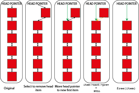
Hopefully the idea is quite clear between the code and the diagrams. If "item" is item "n" in the list then "n-1" is item->prev and "n+1" is item->next. Either or both of these items may not exist if "item" is either the start or the end of the list so you have to cope with these cases. So to update the next element of "n-1" you have to set "item->prev->next" which looks a bit odd but makes sense if you unpack it. Similarly the "prev" element of "n+1" is "item->next->prev".

You will notice that the links on the item being removed aren't touched and the code simply relies on that item being deleted immediately. In a system where you want to retain an item (perhaps to add it to another linked list) you'll probably want to nullify it's prev and next pointers after you remove it from the list.

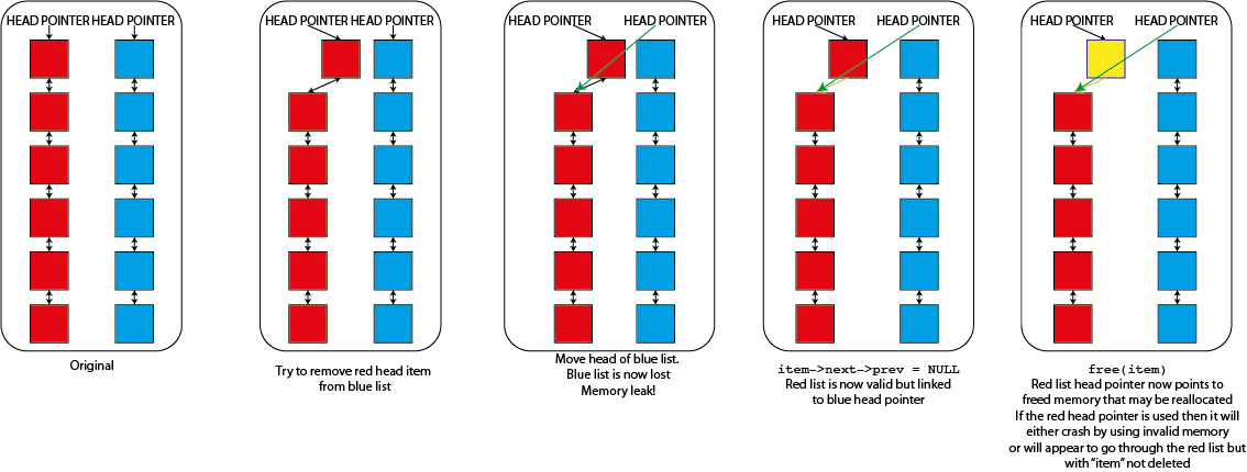
That code will remove any item from the linked list that it is in. There is however a problem if you have multiple lists, each with it's own head element. Imagine that I tried to use that "remove_item" function where I passed it an element from one list but the head from a different list. So long as "item" isn't the first item of the list that it is in then nothing would go wrong but as soon as it is it would replace the head of the second list. This would cause real problems

1. The list that "item" was in will become invalid. Because it's "head" element is never updated it will still point to the now deleted "item" and will sooner or later fail when you try to use it. It might, for a while, look as though "item" hasn't been deleted because of this
2. The original list that you specified the "head" from will now be lost completely. The only reference that you have to a linked list is the head element so if anything happens to this the memory is lost forever. You have both lost data and caused a memory leak
3. You have also moved data. The list that you specified the head from will now be a valid list, but it will be the list that "item" was originally part of, not the list that is meant to be there.

This type of error in a linked list thus causes memory leaks, segmentation faults and data corruption all in one nice package so you have to be careful to avoid it. You can program in safeguards to prevent doing things like this but they do slow down the operation of the linked list and require extra memory (as well as making rather harder some nice tricks that you can do with linked lists that I'm not going to talk about here) so many working linked list implementations don't bother. You can see graphically what's happening here too.

Mostly linked lists in operation are stable and reliable but it is possible to get yourself into a bit of a tangle. But you can immediately see that this makes is a lot easier to remove an element from the middle of the linked list than if you had an array. If you had an array then you'd either have to flag that item as "invalid" somehow to know that you shouldn't use it anymore or failing that actually copy all of the elements in your array above the item being removed down to fill the gap. The first one adds complexity and means that you can't actually reduce your memory footprint when removing items (not quite true if you use an array of pointers to items but that's even more complicated) while the second is quite often very slow. This is especially true if you use a library that guarantees contiguity of the elements of your array after every delete operation when you are deleting multiple items (e.g. std::vector in C++. This behaviour is generally an advantage but here is a cost. You can get around it in other ways in C++ but other libraries are less flexible). The cost is managable if you delete many items and then pack the array up but packing after every deletion can be very costly.

The next entry in this section will describe adding items to a linked list which, as you might imagine, is quite similar to deletion but in reverse.

Christopher Brady : 12 Jun 2019 16:31 |  Tags: Code Programming Training |  Comments (0) |  Close comments |  Trackbacks (1) |  Report a problem

Datastructures – Linked lists part 1

Back to data structures this month with the linked list. Linked lists are a way of holding data that allows you to add and remove items quickly and easily.

Why not arrays?

First question: why is adding and removing items from an array not quick and/or easy? The problem with adding items is quite simple - arrays have a fixed size so eventually you will run out of spaces in your array to store items. When this happens you have to do something to allocate additional space. Many languages have a function called "realloc" or similar that tries to extend the length of your array but it can only do that if there is unused memory space "above" the location of your array because the array elements have to be arranged one after the other in memory. The concept of "space above" is a bit complex in general and depends on details of your OS etc. but as a general idea if you allocate two arrays then they are placed one after the other in the computer's underlying memory so if you try to realloc the first array then there won't be any space between it and the second array to grow it in. If you can't grow your array like this then you have to allocate new memory to store the bigger array and copy the existing elements in. If you keep adding items then this continual growing of your array can be quite expensive, although this can be mitigated by always growing your array by more elements than you immediately need.

Removing items has the opposite problem. Since arrays are required to be contiguous (can't have gaps in them) you can't just "remove" an item you have to either flag it as empty and ignore it when going through your array in future or take all of the items above the removed element and move them down to pack everything up. The first approach has three problems

1. You have to use additional memory to flag items as being empty or not
2. If you are both adding and removing items from your array then since you don't actually recover memory when you remove an item your total memory requirements will grow without bounds
3. Depending on your algorithm you might have more difficulty getting optimal performance if you have to do fundamentally different things for empty and non-empty array elements

The second approach avoids those problems but on average involves copying half of the elements in your array every time you remove an item which can also be quite expensive.

It is quite possible to build a container based on arrays that you can add and remove items from that has good general performance (C++ std::vector is a good example of one) but they always have to make tradeoffs and if you are doing a lot of adding and removing of arbitrary elements it might be better to use a data structure other than an array.

Linked lists

The idea of a linked list is quite simple. Each element in a linked list is like a link in a chain - linked to the item after them, so you go through the linked list by taking the first item then going to the next item and the next etc. until you reach the end. This is generally implemented using pointers in what are often called "self referential structures", that is structures that contain pointers to themselves. These are easy enough to implement in either C/C++ or Fortran.

struct llitem{
  struct llitem *prev, *next;
};

TYPE :: llitem
  TYPE(llitem), POINTER :: next, prev
END TYPE llitem

These are more or less normal types but there is one more important rule: self referential structures can contain only pointers to their own type, not actual instances of their own type (try removing the *s in C or the POINTER attribute in Fortran and it will fail to compile). This is because types, much like arrays, are laid out contiguously in memory so they can only contain things that the compiler knows the length of and if you have a type that contains an instance of itself then there would be an infinite regression problem because you don't know how big it is until you have finished creating it and you can't create it until you know how big it is. Pointers are all of a fixed size so they work OK.

The structure as given is for what is technically called a doubly linked list because it contains links both to the next item and the previous item in the list. A singly linked list has each item linked only to the next item in the list. Doubly linked lists have some substantial advantages over singly linked lists, notably that you can go through it from either end, but also you can remove an item from the list needing only the item itself (and the list that it is held in if you have several).

Creating linked lists

Creating a linked list is quite easy. You hold a simple pointer to the first element in the list (generally called the head item) and then you simply create the list going down from that. The key thing is that you have to hook up the prev and next links as you go. This isn't too difficult and looks like

#include 
#include 

struct llitem{
  int value;
  struct llitem *next;
  struct llitem *prev;
};

void init_ll(struct llitem * l)
{
  l-> value = -1;
  l->next = NULL;
  l->prev = NULL;
}

int main(int argc, char** argv)
{
  struct llitem *head, *current;
  int i;

  head = malloc(sizeof(struct llitem));
  init_ll(head);
  head->value = 1;
  current = head;
  for (i=0;i<10;++i){
    current->next = malloc(sizeof(struct llitem)); /*Create the next element*/
    init_ll(current->next); /*Initialise it to nullify pointers*/
    current->next->value = current->value + 1; /*Simple counter*/
    current->next->prev = current; /*It's previous pointer should be the current item*/
    current = current->next; /*Now move onwards so the newly created particle is now current*/
  }

  current = head;
  while(current){
    printf("%i\n", current->value);
    current = current->next;
  }

}

PROGRAM test

  IMPLICIT NONE
  TYPE :: llitem
    INTEGER :: value = -1
    TYPE(llitem), POINTER :: next => NULL()
    TYPE(llitem), POINTER :: prev => NULL()
  END TYPE llitem

  TYPE(llitem), POINTER :: head, current
  INTEGER :: i

  ALLOCATE(head) !Create the head
  head%value = 1
  current => head
  DO i = 1, 10
    ALLOCATE(current%next) !Create the next element
    current%next%value = current%value + 1
    current%next%prev => current !The next element's previous is the current element
    current => current%next !Now move onwards so the newly created particle is now current
  END DO

  current => head
  DO WHILE (ASSOCIATED(current))
    PRINT *,current%value
    current => current%next
  END DO

END PROGRAM test

This example also shows how you how to step through the linked list from the head, simply by having a "current" pointer that starts at head and is then incremented by setting current = current->next (or current => current%next in Fortran). This can look a bit odd but it isn't that hard to understand. I start by manually creating the "head" element, using either ALLOCATE or malloc. Once I have a head element I then loop through, each time using the same ALLOCATE or malloc command on the "current->next" pointer, creating a new item every time. In C I then call the ll_init function to setup the values of the struct (in Fortran this is done for me since I gave the elements of my TYPE default values). After this the prev and next pointers are both NULL. This is correct for the next pointer becuase my new item is the last item in the list (it won't be next iteration but right now it is), but I have to set the prev pointer. If my new item is the next element in the chain from my current element then the previous element in the chain from my new element must be my current element so I set that up. After that I just have to repeat until I have added enough items.

Part 2 of this will be in a couple of weeks and will describe how you remove and item from a linked list and how to add new items to the middle of a linked list.

Christopher Brady : 15 May 2019 17:20 |  Tags: Code Programming |  Comments (0) |  Close comments |  Trackbacks (1) |  Report a problem

Pretty please print

The possible impossible

A pretty short entry this week, on a likely familiar theme. You have some buggy code. You try and trace the bug by inserting 'print' statements. Eventually you have prints wrapped around the troublesome piece and you may find yourself saying something like:

Aha! It reaches line A, but never line B! But thats IMPOSSIBLE! There's nothing there but simple code that can't just not execute! In fact there's only blank lines!

As usual, once you find yourself uttering a line like that, it's time to step back. Computers only rarely do the impossible.

Many things can have happened here, but a common, very confusing one, is that the second print has run, but you're not seeing the result. This is common because most languages default to bufferredoutput to stdout. We mentioned this a little bit in context of output streams in a previous entry, here we give a bit more detail.

Aside - stdout

If stdout and stderr aren't already familiar, they are the short names for standard out and standard error. There's a little bit about those herebut basically they are the designated way of writing output (information) and errors to the terminal. They're separate because sometimes you only want to see one or the other. You can direct them to separate files if you want (see the link for how). It is very good practice to respect the designation, and use the correct stream when you write information. It's acceptable to write everything to stdout in your code, but you really shouldn't be writing anything except actual errors to stderr. Warnings are acceptable, but only if they're "important". Save it for things that a user really needs to know.

Back to the Print Problem

The conversation goes something like this:

"So, what's going on with my prints? If it's printing but I don't see it, where is it?"

"It's in an output buffer, waiting until there's enough stuff to be worth printing. "

"Hang on, worth printing? I think it's worth printing! Print it!"

However, there is a good reason. The easiest way to show this is with some code. The following Python3 code uses both buffered output and unbuffered output where we force each print statement to flush the buffer so each print happens exactly as it is reached:

import time
_iters = 100000

def many_prints(flush):

  for i in range(0, _iters):
    print(i, flush=flush)

start_time = time.time()
many_prints(False)
timef = time.time() - start_time

start_time = time.time()
many_prints(True)
timet = time.time() - start_time

print("No flushing --- %s seconds ---" % timef)
print("Flushing --- %s seconds ---" % timet)

Run this a few times and you should see that flushing is slower. It's not always by much, but it can be 20%, or more, depending on system, which is sometimes significant.

Why so Slow?

So why is unbuffered output slow? In this case, mainly because interacting with the terminal and redrawing the screen takes time. Writing to a file can be even slower, because now we have to interact with the file system and disks, and maybe even wait for a success signal to come back. It's much better if these events can be collected into larger bursts, so we only have to do that rigamarole once.

Unbuffered Output and Flushing Options

We showed Python3 above, where we can simply use the flush Keyword. In Python 2 we have to do a little more. This linkshows the main options. We can force the Python interpreter to not use buffering at all, or we can override it for given output streams. Or we can write custom objects that flush exactly when we want.

In Fortran, we just call the FLUSH subroutine either on all outputs or the unit of our choice.

In C, we can flush stdout with fflush, set stdout to be unbuffered, or use stderr which is unbuffered by default.

In C++ there is a slight wrinkle as we can use either C-style IO via stdio, or C++ streamio. std::endl is a command to flush the output stream, not just a new-line, so it's usually recommended to use `'\n' to get just a newline, and std::endl only when required.

C++ IO

While we're here, we should mention on thing about mixed IO in C++. By default, a program can mix stdio via printf and stream-io (using <<), and similarly for input. BUT these two methods have to be force to share any buffering, or else the would not work together. This means they are forced to stay in sync, so inputs and outputs work as expected. In some circumstances, especially if a lot is written to stdout, it may be useful to only use one or other of these, and disable the syncing. See here for details, but be very very careful.

Bottom Line?

The bottom line of all of this is pretty simple. When doing print-style debugging, or printing error messages, either use stderr (making sure that's not buffered in your language or system), or flush after every essential stage of your prints, or disable buffering completely while debugging. You don't need all three. And finally, remember the golden rule. If it looks impossible, you're probably assuming something that isn't true. Not terribly snappy, but a useful thing to remember.

Heather Ratcliffe : 03 Oct 2018 21:16 |  Tags: Code Debugging Io |  Comments (0) |  Close comments |  Report a problem