All 14 entries tagged Programming

Again and again and again

"Flow control" means all the ways you can control what your program does, both now and next. Conditionals, loops, function calls all count. Exceptions (throw, raise etc) may or may not - whether its OK to use exceptions as flow control or whether they're meant for, well, exceptional occurences (not necessarily rare, but something that can't be handled by the current piece of code) is a seriously vexed question.

Loops

Loops are usually the first or second control option to be taught, and take two general forms, the 'for' type loop and the 'while' type loop. Different languages use different words, but the first one is meant to do something a certain number of times, and this number is known when the loop starts. The second is meant to do something 'until told to stop'. This is not a hard distinction though. A while-type loop can always mimic a for-type loop, and the reverse is also true (although sometimes considered to be inelegant and/or error prone).

Usually, these loops look like

For index = start to end
   {loop body}
End for

and

While condition
  {loop body}
End while

The condition can be as complicated as you like, it just has to evaluate to either True or False. It can use all the variables you might be changing in the loop, etc. So we create the other kind of loop something like this:

For index = start to max_iterations
  {loop body}
  If condition exit_loop
End for

and

index = start
While true //This means keep looping forever
  {loop body}
  If index > end exit_loop
   index = index + 1
End while

Note that whether we get (end-start) iterations of a for loop, or (end-start+1) or (end-start-1) can vary by language, but we can easily adjust to match.

Recursion

The other way of doing something many times, is 'recursion'. This often gets classed as 'super advanced and difficult' for some reason, but is mostly quite simple. First though, we need to know a tiny bit about functions and how they're called.

Scope

Scope is very, very important: every variable, function etc within a program has a scope. For variables this means "parts of your code which can use this variable (bit of memory) with this name". For functions, it means "parts of your code which can use this function with this name". There's a few subtleties beyond that, but for now, this will do.

So, what scopes are there? A variable defined inside a function is only usable within that function: it is scoped to that function, or has 'local scope'. A variable defined globally (outside any functions, including main) has 'global scope' and is available everywhere. Do note that a variable defined in 'main' is only available in 'main' and NOT in any functions 'main' may call, as main is a function like any other.

Most languages also have an idea of 'block scope' where 'blocks' (in C anything inside curly braces {}) can contain variable declarations, which are only available inside the block. This can cause some particularly confusing errors, such as when you try and do the following:

while i < 10 
  int i
end while

which will not compile unless there is already a variable, called i, and the one you declare inside the loop then 'shadows' this - inside the loop i refers to one variable, outside the loop, including the loop condition line, i refers to something different. If this isn't completely clear, the following example should help:

string name = 'Nobody'
int i
for i = 1 to 3
  string name = get_string_from_user() 
  print i, name
end for
print 'You entered', name

which gets 3 names from the user an outputs something like:

1 Bill Bailey
2 Madonna
3 Engelbert Humperdinck
You entered Nobody

Another tempting thing is to try

if condition then
  int i = 0
else
  long int i = 1
end if
print i

which again has either an undefined 'i' or a shadowing problem. There is no way to get a different type for i using an if like this, and with good reason. i's type could only be determined in general when the program runs - so how much storage should be given for it, and can it be passed to any given function?

Function scope has one more really important thing though - each call to a function is a new scope. The variables you used last time do not keep their values.

FORTRAN PROGRAMMERS - READ THIS!!!

In Fortran there is one really important idea called the 'SAVE' attribute. A variable in a function (or module) can be given this, as e.g. "INTEGER, SAVE :: a" and the value of 'a' will be kept from call to call. This is very useful. BUT there is a catch. Any variable declared and defined in a single line in a Fortran function is given the SAVE attribute. So, if you do something like `INTEGER :: alpha = 0`, declaring an Integer alpha and in the same line defining it, alpha is set to zero ONLY the first time the function is called. Subsequent calls will inherit whatever value alpha had last time. This is rarely what you intended. Be careful!

Call stack

When you write code to call a function, the computer has to stop what its currently doing, and enter a new scope containing only the variables available inside the function. It also has to remember where it should go back to after the function ends. This is done using the 'call stack'.

We haven't talked about 'stacks' as a data structure yet (coming soon) but we did mention here that they're a "last-in-first-out" structure where the last thing you add to the stack (think of a stack of papers or books) is the first one you take off. Each time you call a function, you add an entry to the stack, and when you return this is 'popped off' and the stack shrinks. Each entry is called a 'frame'.

The stack frame usually contains the location to return to, and also memory for all of the local variables in a function. It often also has space to hold all the parameters passed to the function and sometimes a few other bits of operational stuff. When a function is called, a frame is created with all this in, and when it returns this is destroyed.

We mentioned above that variables inside a function are available only inside it, but we didn't ask what happens if we call a function from within itself. We've seen that between calls to a function the values are 'reset' or lost, and having read the previous paragraph you probably guess that this is both because and why the stack frame gets destroyed.

Now, you might suggest that you could always make sure every call to a given function shares the same variables, but if you've ever used a function pointer you know that you can call a function without ever using its name at the place the call actually happens, so this isn't practical. So, each call to a function, any function, creates a stack frame containing all its local variables, and calling a function from within itself makes two, independent, sets of all the local variables, that know nothing about each other.

My First Recursive function is My First Recursive function is My First....

So what is recursion then? "Recursion occurs when a thing is defined in terms of itself or of its type." (Wikipedia, Recursion) For a function, recursion means having the function call itself. In maths, the factorial function of a number which is the product of all positive integers up to it. So we see immediately that factorial(n) is n*factorial(n-1), which we'd code up something like this:

function factorial(integer n)
  return factorial(n-1)*n
end function

We can pretty immediately see a problem there though - how does the chain ever end? We need something which is not recursive or we'll go on calling forever. This is called the 'base case' and for factorial its obvious from how we said 'positive numbers'. The function above won't stop when n = 1 and it should. So what we actually want is:

function factorial(integer n)
  if n > 1
    return factorial(n-1)*n
  else
    return 1
  end if
end function

Follow this by hand, on paper, for a starting n of say 4. We enter factorial(4), which enters factorial(3), which enters... until we reach factorial(1), which immediately returns '1' to the layer above, factorial(2), which multiplies this by '2' to get '2' and returns this to factorial(3) and so on.

Each Call is Its Own Scope

Remember when looking at recursive functions that each layer of call is a separate scope, with a separate copy of any variables you may define. Anything which needs to go between the layers has to be passed as an argument.

Step by step by step

So we have these two ideas that both let us keep going until we reach some condition, namely recursion and a while loop: what's the difference. There isn't one. Anything you can do with a loop you can do with recursion and vice versa. There are differences in elegance, and often one is a better choice, but not more. In fact some functional languages don't have any concept of the loop, relying solely on recursion. Mostly, elegantly recursive problems are better written as 'while' type loops and rarely as 'for' type loops, because the base case is the same as the loop-stop condition. Some recursive problems, usually those involving trees, are very hard to do elegantly with a loop.

Induction

Most of programming is about working out the sequence of steps to get from A to B, so that what you actually code is just a series of things, one after the other. Sometimes these steps are completely independent, and sometimes they aren't but they always (in a single-threaded program) run one after the other. We're always having to think about things, not in terms of the big picture, but just in terms of getting from here to there, ignoring how to get here in the first place.

In maths, one of the simplest methods of proof is called 'induction' which is closely related to recursion. Rather than try and prove the 'whole of a thing' we say 'if it was true for a smaller thing, can we show it's true for the next larger thing?' and then we say 'can we prove its true for the smallest thing?'. If we can do both of these, we've shown its true. As used here a common example is climbing a ladder. We say 'can we climb onto the bottom rung?' and we say 'can we climb onto the next higher rung than we're on?' and if so, we can climb any ladder.

Sometimes, a slightly stronger assumption is used where we instead say 'if we have reached every rung below and including the one we're on, can we reach the next one'. This is actually equivalent, but is sometimes a more useful phrasing.

Proofs by induction only work if it doesn't matter which rung we're on to climb to the next one. We don't ever have to reach rung 53 to know we can reach rung 54. If you have a problem which is easy to think about this way, then it is a prime candidate for programming recursively. The step is always the part going from 'here' to the next 'there', and the base case is how you get to the first 'here'.

Problems with Recursion

Stack Overflow

The 'call stack' we've been talking about is the inspiration for the programming forum Stack Overflow which is probably the most encountered error when programming recursively. Each function call creates a call stack frame and there is a limit to how much memory is available for this. If you forget or mis-program the base case, your recursive function never stops calling itself, until it has filled the call stack and your program crashes horribly with a stack overflow.

The other common way to get a stack overflow is creating large temporaries inside functions since these are all part of the stack. Hopefully more on that soon.

Function Parameters

Secondly, recursion can be a bit tricky to actually set up. Our factorial function was nice and simple, with a single parameter, and a single return value. But what if we have more than one parameter? For instance, a binary search can be done nicely in recursive fashion. Each step is about deciding which half, upper or lower, our target is in, and passing only this half on to the next step, and the base case is when this has length 1. Here though, you want to pass at least two items - the segment of list, and the target value, and you want to return either true or false, or the index the target was found at. If returning the index as an offset into the passed segment, you then have to adjust this at each step so that you end up with the index in the original, complete list. This can get mucky.

Excess Work

The other common example used for a recursive operation is the Fibonacci sequence where the nth value is the sum of the (n-1)th and the (n-2)th. Usually, the first two values are 1, so the sequence goes 1, 1, 2, 3, 5, 8, 13 etc. It's not hard to write a recursive version of this, e.g.

function fibonacci(n)
  if n eq 1 or n eq 2 
    return 1
  else
    return fibonacci(n-1) + fibonacci(n-2)
  end if
end

but if we work through this on paper for say n =5 we find that we calculate the n=4 case once, the n=3 case twice, the n=2 case three times and the n=1 case twice.

A Python version of this and my model answers to the challenges are here.

Challenge: what's the rule in general for how many times fib(m) is called for each m < n?

Challenge 2: rewrite this recursively with exactly n-1 calls to calculate fibonacci(n). Hint after the post, or solutions at the Github link above.

If we're not careful, we might never notice all the extra work we're doing, which we could avoid. In this case, there's a big hint that something is funny at the point where we put two values of n into our base case.

Challenge 3:

Some image sharing sites now try to use a few real words to create memorable random urls. If you're given n lists of words, can you write loop based and recursive variants of the code to create every combination of one word from each list? Your code should work for any value of 'n'.

For example [large, small] [radiant, lame] [picnic, bobcat] should give (order not important) large-radiant-picnic, small-lame-bobcat, small-radiant-bobcat etc etc.

Small hint below the post

Moral of this Post

The takeaway from this one is that recursion isn't scary if you just think about getting from here to there, pretending all the business to get 'here' has been dealt with. Never mind the rest of the ladder, just think about the next rung. This is one of the vital skills to develop as a programmer, on every scale. Break things down into manageable steps and then build them into a program.

Keep scrolling for the hints....

Hint 1: can you return both the (n-1) and the (n-2) values?

Hint 2: the list created by combining lists 1 and 2 is itself a list of words. 3 lists is just 2 lists, and then another list.

Heather Ratcliffe : 13 Feb 2019 17:24 |  Tags: Flowcontrol Programming Soup |  Comments (0) |  Close comments |  Report a problem

Data structures – Queues

This week we're back on data structures with another fundamental one: the queue. Simple data queues are pretty much the same as queues in real life, new items arrive at the back of the queue and data is removed from the front of the queue. They have obvious applications in any kind of program that gets data in from an external source and then has to process it in the order in which it is received. Queues are what are called FIFO data structures, first-in-first-out, because the first data to arrive is also the first data to leave. The alternative LIFO (last-in-first-out) data structure is generally called a "stack" because it is much more like stacking up paper in that the last item that you put down is the first that you pick up again.

The easiest way to implement a queue is using an array combined with a front and a back marker (I'm going to stick with the neutral "marker" description because the general idea doesn't care if you use array indices or pointers or any other mechanism that you want to). The idea is quite simple. You start with an array and when a data item turns up you insert it at the back marker and then move the back marker on one element. Adding an element to a queue is often called "pushing" or "enqueueing" so you might encounter those terms. Schematically, this looks like

When a piece of data is requested from the queue you return the item under the front marker and then move the front marker on by one. This operation is also known by the terms "pop" and "dequeue" so those are also worth remembering.

And you continue doing this, moving the front and back markers as data arrives and leaves.

So far, so good but there are two obvious problems. The simpler one is what happens if data is requested when no data is in the queue. You have to have some mechanism for dealing with this case by indicating that there is no data available but that isn't too hard. The more troublesome one is what happens when the back marker goes off the end of your array? In the case as show, you can't really do anything at all and one way or another the queue will fail. This type of queue implementation is only useful if you have a fixed known number of items that you need to store as they come in and then deal with. It's not much use for getting data until your program stops and dealing with it.

If you want to do that, there are a few general solutions

1) You can get rid of the front marker entirely. Every time you dequeue an item you take the first item in the array and then simply shuffle the other items down one so that the first item is always populated so long as there are any items in the queue. This works well but it does potentially involve a lot of copying or moving of data if you have a large array that is mostly filled since every element of the array has to be shuffled up by one. If you are dealing with objects where a move/copy operation is expensive or are dealing with threaded code where some threads have to wait while this happens then it isn't the best solution

2) You can move to a circular queue. Circular queues are a bit strange and break the analogy with real world queues since queueing in a circle doesn't really work in reality. The idea is pretty simple though. Since you knowthat everything to the left of the front marker is unused, why not put new elements into there as they arrive and move the back marker around with them? Then when the front marker reaches the end of the array it just goes back to the beginning too. The effect is to mean that the front marker chases the back marker round in a circle. Shown schematically, this looks like

This works so long as back never catches up with front. If it does then either it has to stop adding data or it will overwrite data that is already there. It is possible to generalise these two examples to an arbitrarily long array - simply create a new array that is longer and copy the extant data into it and start again - but in most of the situations where you want a queue it should be possible to avoid this since that is another expensive operation (that will also render any pointers that you have to your data invalid so might involve more work to sort out pointers).

Generally queues are used in producer/consumer systems. There is something that is producing data and something else that is operating on it in some way. On average you have to be operating on the data at the same rate as you are producing it or the data will build up without limit, so the queue is only there to buffer data for brief periods while either your producer produces data faster than normal or your consumer consumes it slower than normal. In this case, all that you need is a large enough queue to deal with the largest expected difference in production and consumption rates. Of course, in a lot of systems you can only predict that "this queue is large enough for 99% of the expected variation" so for the other 1% of the time where you run out of space in your queue you have to decide whether it's worse to stall your entire system while you make your queue bigger (this might be OK for a web server for example where a page might take slightly longer to load but otherwise would work as expected) or simply throw away data (for example in a data logging system where any halt in the process would cause data loss but it might be lower if you just throw it away until there's space to store it than waiting while memory is allocated to hold it). Unfortunately, which is the right answer depends very much on the problem that you are working with.

As a final note, there is also a very similar data structure called the double ended queue or deque (pronounced "deck") that is similar but allows you to add and remove data from either end of a queue. They behave very similarly in general but the implementation gets a bit fiddlier because your back and front markers have to do double duty as each other.

Christopher Brady : 30 Jan 2019 17:39 |  Tags: Programming |  Comments (0) |  Close comments |  Report a problem

Searching in data

One of the most common things that you'll want to do in programming is to look in a list of items to find out if a given item is in there. The obvious way of doing it is by going through every item in the list of items and comparing it to see if the items are the same. On average, searching for a random item in a random list of items you'll have to look through half of them before you find the item you want (obviously sometimes you'll find your item quicker than this, sometimes you'll have to look through all of them before you find the one that you want. But on average over a very large number of searches you'll compare half of the list on each search) This algorithm is generally called linear searchboth because you go through your items in a line, one after the other, and because the time that it takes is linearin the number of elements. By this I mean that if you double the number of elements in your list it will take twice as long (on average) to find a given element. In the normal notation of algorithms this is called O(n) "order n" scaling (this is one use of so called "Big O notation"). If doubling the number of elements would take four times as long (quadratic scaling) you'd say that your algorithm would scale as O(n²) "order n squared".

In general, there is no faster way of finding a random element in an unordered list than using linear search. On the other hand, if you have an ordered list then you can speed things up by using bisection. The idea is quite simple. Imagine that you have the first seven entries in the International Radiotelephony Spelling Alphabet (IRSA, don't worry it's probably more familiar than it's name!) in order

Alfa
Bravo
Charlie
Delta
Echo
Foxtrot
Golf

and you want to find the item "Bravo". Obviously, by eye this is easy but you want an algorithm that a computer can follow. You know that you have 7 items, so you compare the item that you want "Bravo" with the one at the half way point "Delta". You know that "Bravo" is before "Delta" in the IRSA and because you know that your list is ordered you can then throw away everything from and after "Delta".You now have

Alfa
Bravo
Charlie

,three items. Once again, check the middle one, which this time is "Bravo" so yay! You've found your target in your list, and it only took two tests despite there being seven items. This is because every time you make a comparison you can throw away half of your list, so doubling the length of your list doesn't double the number of operations that you need, it actually only (on average over all possible lists) adds a single additional operation. Technically this algorithm is O(log(n)) "order log n", which makes it very, very useful if you have a large number of items. Imagine that you have 256 items, you'd have to compare all 128 of them (on average) in linear search compared to 8 (on average) in a bisection search. If you go to 4096 items then it gets even more extreme with 2048 comparisions for linear search compared to 12 for bisection. Similarly if your target item was "Foxtrot" and after "Delta" then you could throw away everything before and including "Delta". By alternatively throwing away either the top or the bottom of your list you always get to the item that you want.

As always though, there are problems. First you have to be able to access any element of your list freely. I quite happily said 'compare the item that you want "Bravo" with the one at the half way point "Delta"' without asking how you go from "half way point" to "Delta". While we haven't covered them yet there are some forms of data structure (notably linked lists which we'll cover soon) where you can't easily do this kind of hopping around inside your list and bisection is usually much less efficient or impractical in these kinds of data structure.

Second, this really does onlywork on ordered lists as you can clearly see by the way in which I just threw away half of my list based on the property of the middle item. You might be tempted to say "ah! I can just sort my list" and indeed you can, but even the best algorithm for sorting a list is O(n log(n)) "order n log n", which in general means that it is just a bit slower than a linear search through your data. What this means is that it's only worth sorting your data and then using bisection to search in it if you're searching in your data much more than you are adding to it, so you can sort your list once and then do many searches on it before it becomes unsorted again when you put new data in. This general idea (although not always the details) is the idea behind indexesin databases. You create ordered lists of data that you want to search on a lot so that you can find the data that you want quickly.

Bisection is a very general approach that you find in all sorts of problems, not just finding items in lists. The general idea is the same : throw away half of you items because you know that the item that you want cannot be in that half.

Christopher Brady : 17 Oct 2018 17:45 |  Tags: Programming |  Comments (0) |  Close comments |  Report a problem

Upcoming Training Opportunities

Warwick RSE's autummn term training is now available for signup for any University of Warwick Staff or students, and anybody from the HPC-Midlands-Plus consortium.

This time we have two options.

The first is aimed mainly at Warwick Researchers who wish to use HPC facilities. We'll go through getting access and some essential info you'll want to know, as well as briefly mention where else you can get computing resources.

Secondly, we have a short 3-hour seminar going over all the bits of Software Development researchers should know about. This will be a pretty rapid spin through a lot of tools and words you'll need to know. Hopefully, you'll then spot when you should go and learn more about these things as they come up in your research etc.

For dates, signup etc, see our calendar

Heather Ratcliffe : 02 Oct 2018 17:41 |  Tags: Hpc Programming Training |  Comments (0) |  Close comments |  Report a problem

Scheduling and processor affinity

We're taking a brief break from data structures to talk about something a bit different : scheduling and processor affinity. This is dealing with a problem that a user or developer doesn't usually think about, but is crucial to the performance of modern computers. Describing the problem is quite simple : if you have a computer that is doing multiple tasks what order should they happen in and what processor (if you have more than one) should take on each task? Working this out is the preserve of the very core part of the operating system (OS), generalled called the kernel (after the part of the nut). While the term is most familiar from the Linux/Unix world (technically Linux is the name for just the kernel and not the rest of the OS), macOS has the Mach microkernel at it's core and ntoskrnl.exe (the Windows New Technology Kernel! It was new in the mid 90s at least) is at the core of modern versions of Windows.

The simplest solution is for the kernel to just create a queue of programs that have to be done and then run them one after the other, with each new program being handed to the next free processor and programs running until they are finished. This is typically called First In, First Out scheduling (FIFO, which is a very common acronym in computing. Do not confuse this with GIGO (garbage in, garbage out) which is also a very common acronym in computing). FIFO scheduling works very well for computers that are working on lists of tasks having equal priority. So batch processing of data for example works very well with FIFO scheduling. But you can immediately see that it won't work well for all computers that humans actually work with interactively. If all of your processors are working on long, slow processes then your computer would stop working completely and you wouldn't even be able to stop the processes because the computer wouldn't be processing your keyboard or mouse input.

Normal computers tend to work using a system of preemptive scheduling. This works by taking a program and letting it run for a while on a processor and then saving its state, stopping it and then giving the processor another program to run on that processor for a while until stopping it etc. etc. Eventually you get back to a process that has been running before and you restore it's state and start it running again. Because the state of the program is stored completely it is entirely unaware that this has happened to it, so it just runs on regardless. (as a historical note, this is called preemptive scheduling because the OS kernel preempts the programs running on it. It basically says "you're done, get out of the way" and lets other programs run. Older systems used cooperative scheduling where a program would have code in it where it said to the kernel "I'm ready to be switched away from". This worked fine until a badly behaved program didn't reach this point whereupon every other program on the computer stopped working.)

There are disadvantages to preemptive scheduling. The saving and restoring of the state of programs is generally called "context switching" and it does take time for this to happen. (FIFO schedulers don't have this problem because programs run until they complete, but even now you can't really use FIFO schedulers because there tend to be dozens of programs running on a computer at once and some of the effectively nevercomplete until the computer shuts down). If you only have one processor then context switching is the inevitable price of allowing multiple programs to run at once, but if you have two processors and two programs then they can happily run alongside each other so long as they are each running on their own processor.

But what if you have four programs and two processors? As you'd guess, in general you'll put two programs on each processor. But what happens if the processors aren't running through their jobs at quite the same rate? This can happen because real schedulers are rather more complex than I suggested here. In that case, you can come to a situation where the program that was running on processor 1 reaches the point where it should run again but processor 1 is still busy. Should it then be run on processor 2? The answer, is "maybe". Sometimes programs benefit a lot from data being held in the fast CPU cache memory and if it now runs on a different processor then that benefit is lost. Under that circumstance it would be better to keep that program running on the same processor even if it has to wait a bit longer until it runs again.

All common operating systems let you do this and it is called "processor" affinity. You tell the kernel which processor (or processors) you want a given program to run on and it guarantees that it will respect that rather than giving that program to the next available processor.

I've glossed over a lot of things about scheduling here (in particular Intel's Hyperthreading technology is a nightmare for scheduling because it creates "virtual" processors to try and take advantage of the fact that most programs don't use all of the parts of a processor at once. The problem is that these virtual processors don't behave the same way as real processors so the scheduler has to be much more careful about what programs it should run on them.), but this is a decent overview of how scheduling and process affinity works on modern computers and generally it works quite well. General purpose programs don't set CPU affinity and just run as quickly as possible when a processor is free, and programs that do heavy numerical computation set CPU affinity to try and maximise cache performance. But there are interesting cases where it can fail.

Recently we had an interesting discovery using the OpenMPI parallel programming library. This is a distributed programming library intended to write programs to run on large "cluster" computers that consist of lots of single compute nodes connected by a network. But it does also work to run programs on a single computer. We were testing a computer with 16 cores and found that running a single 16 processor job was about 16 times faster than the same problem on a single core. When we tried the same problem with 4 simultaneous 4 processor jobs things were very different. The 4 processor jobs were all slower than they were when running on a single core. After a couple of hours we found out why: OpenMPI sets processor affinity for all of the programs that it runs, but it always sets them for the lowest numbered processors. So running a 16 core job ran them on cores 0 to 15, but running 4 sets of 4 core jobs ran them allon processors 0 to 3, so they all basically got a quarter of 4 cores. Add in some overhead from context switching and you get that it's slower than running on a single core. One quick parameter to the library to tell it not to use processor affinity and we were back to where we expected to be, but the lesson to take away is that you can get far to used to things like schedulers just working. If you're finding that things are running slower than you expected, check whether or not there's something odd going on with how your processors are being used.

Christopher Brady : 19 Sep 2018 17:16 |  Tags: Programming |  Comments (0) |  Close comments |  Report a problem

Data structures 2 – Arrays Part 2

Part 2 of arrays is about dynamic (run time) sized arrays. That is arrays where you don't know how large they're going to be until the code is running. First, I'll go through it in Fortran because it is really easy in Fortran, and powerful array operations are one of the major advantages of Fortran.

Dynamic arrays in Fortran are generally called ALLOCATABLE arrays (there are also POINTER arrays, but they are generally harder to use for only fairly specific benefits), and you declare them pretty much the same way that you declare any array in Fortran

INTEGER, DIMENSION(:), ALLOCATABLE :: myarray

You then allocate it using

ALLOCATE(myarray(0:100))

First, note that the DIMENSION(:) syntax in the variable declaration is the same as when you're passing an array to a function where you don't know how big the array is. This is the general way of telling Fortran "I don't know what size this is until runtime" (there are a few features where it's * instead for things like the length of strings, but in general it's :). Also note that I have explicitly allocated the array bounds, with the array running from 0 to 100 inclusive. If I'd just used

ALLOCATE(myarray(100))

then the array would have run from 1 to 100 inclusive. In Fortran you can have any upper and lower bounds for arrays that you want which is sometimes useful. You do have to be careful though because unless you are careful when you pass arrays into functions these bound markers are ignored inside the function and the array just runs from 1:n.

Moving to multidimensional arrays in Fortran is easy.

INTEGER, DIMENSION(:,:), ALLOCATABLE :: myarray
ALLOCATE(myarray(0:100, -1:101))
myarray(10,10) = 1

will create a 2D column major array with the array bounds that I specified in my allocate statement. Job done. Fortran ALLOCATABLE arrays also have the nice property that they are automatically deallocated when they go out of scope so it's much harder to have memory leaks with Fortran ALLOCATABLE arrays (you don't have this guarantee with POINTER arrays because this doesn't make use of reference counting and garbage collection. It relies on the fact that there can only be a single reference to a Fortran allocatable.). If you want more control over when memory is returned to you then you can also manually DEALLOCATE the array

DEALLOCATE(myarray)

Before I start on the C section, I should note one thing: C99 and later standards do define variable length arrays (usually referred to by the acronym VLA). They aren't really very common in scientific code and they have all sorts of oddities about how you use pointers to them and where you can and can't use them (you can't have them in structs for example). Given their general rarity and strangeness (and the fact that they aren't valid in C++ before C++14) I'm not going to talk any more about them, but they do exist and you might want to look them up if you're writing a new code in C. 1D run time arrays in C are traditionally created using the "malloc" memory allocation function. You tell malloc how many bytes of memory you want and it creates a chunk of memory that long and hands you a pointer to it. The syntax is easy enough

#include <stdlib.h>
int main(int argc, char **argv){
int * myarray;
myarray = malloc(sizeof(int) * 100);
myarray[0] = 10;
free(myarray);
}

Note the use of the "sizeof" operator to find out how many bytes are needed to store an integer. If you want to write code that works on multiple machines you'll have to use this because integers are not always the same size. In most senses you can consider a pointer and a 1D array to be very similar in C. When you use the square bracket operator you get the same element of your array in both cases, and in fact the layout of the memory behind the scenes is conceptually similar (although if you want to be precise a static array will generally be allocated on the stack, while malloc gives you memory from the heap). Also, note that I have used the function "free" to delete the memory when I am finished. If I don't do this then there will be a memory leak. C explicitly does not keep track of memory at all. Sadly it gets rather harder in multiple dimensions.

malloc always gives you a 1D strip of memory, and there is no equivalent function to give you a multidimensional array in standard C. My preferred solution is just to allocate a 1D array and then use an indexing function to access the element that you want. For example

#include <stdlib.h>
int main(int argc, char **argv){
int * myarray;
int nx, ny; /*Size of array to be filled somehow*/
int ix, iy; /*index of element to access to be filled somehow*/
myarray = malloc(sizeof(int) * nx * ny);
myarray[ix*ny + iy] = 10;
free(myarray);}

This will work perfectly and will give pretty good performance. Usually you'd write some kind of helper function or macro rather than having ix*ny+iy all over your code, but this shows the general technique. You do have to be careful writing your index function though because [ix*ny + iy] gives you a row major array and [iy*nx + ix] gives you column major. This can be useful but you need to be sure what you're doing. The other problem with this is that you can't just access your array as if it was a compile time multidimensional array. If you try to access this using myarray[ix][iy] you will get a compile error. This is because behind the scenes the [] operator dereferences your pointer with an offset (you can replace myarray[ix] with *(myarray+ix) if you like pointer arithmetic). Because of this when the first square bracket has happened you are just left with an integer, so the second square bracket operator is an invalid operation. So can you keep the multidimensional access? Yes, but there are always downsides.

#include <stdlib.h>

int main(int argc, char **argv){
int **myarray;
int nx, ny; /*Size of array to be filled somehow*/
int ix, iy; /*index of element to access to be filled somehow*/
int ind; /*Loop index*/
myarray = malloc(sizeof(int*) * nx);
for (ind = 0; ind<nx;++ind) myarray[ind] = malloc(sizeof(int) * ny);
myarray[ix][iy] = 10;
for (ind = 0; ind<nx;++ind) free(myarray[ind]);
free(myarray);}

This works by making myarray a pointer to a pointer to an int (int **myarray). You then allocate the outer pointer to be an array of nx pointers to int (note that my first sizeof is now sizeof(int*), not sizeof(int)!). You then go through all of these pointers to integers and allocate those pointers to themselves be ny element long arrays of integers (note that the second sizeof is sizeof(int)). This will work as expected, and you can now index your array with square bracket operators as normal, so what's the problem. The problem is that malloc doesn't give any guarantees about where the memory that you get back from it is located. In this simple test case the memory that you get will probably be layed out in a contiguous block, but in general this won't be true. By splitting your memory allocation up like this you are potentially creating a memory prefetch problem much like the one that you get by accessing an array in the wrong order, with similar effects on performance. There is a fringe benefit for this type of array : because the rows are allocated separately they don't have to be the same length as each other. It's tricky to make use of this property (because you have to keep track of how long each row is yourself) it can be very powerful for certain types of problem. On a related note you will often find that multidimensional arrays in C++ are created using std::vector<std::vector<int>> types. This in general has the same type of problem with memory not being contiguous, as you can clearly see from the fact that you can push back into each vector individually.

The final solution is to create a 1 dimensional chunk of memory and then rather than using an indexer function use a separate list of pointers to the start of the row. There are lots of ways of doing this, and this example isn't a terribly clever one but it does work

#include <stdlib.h>

int main(int argc, char **argv){

int nx = 10, ny=10;
int ind;
int **myarray;
int *buffer;
myarray = malloc(sizeof(int*) * nx);
buffer = malloc(sizeof(int) * nx * ny);
for (ind = 0; ind< nx; ++ind) myarray[ind] = &buffer[ind * ny];
myarray[5][5]=54;
free(buffer);
free(myarray);}

Christopher Brady : 05 Sep 2018 17:18 |  Tags: Code Programming |  Comments (0) |  Close comments |  Report a problem

Data structures 1 – Bitmasks

This month we're going to start an occasional series on data structures. Data structures are one of the core foundations of computer science, but are often underappreciated by general academic programmers. A large part of this is simply that data structures are usually chosen early in development of a code and are only rarely changed as the code evolves. Since most people don't start a code themselves, but simply work with an existing one, you only need to know how to work with a given data structure rather than why it was chosen or why it's a good choice. To try and remedy this we are going to create a few blog posts on common data structures, why they are chosen and how to implement them.

The first one is definitely one from the archives, being a trick that was more useful when computers only had a few kB of memory available to them, but is still used in modern codes because of it's simplicity. This month, we're going to be talking about bitmasks.

Bitmasks

Bitmasks are solutions to the problem of you having a large number of simple logical flags that you want to keep track of and keep together. The common uses are things like status flags (what state is this object in), capability flags (what can this object do) and error flags (which errors have occured). The answer seems obvious:

LOGICAL, DIMENSION(N) :: flags !Fortran
std::vector<bool> flags; // C++
char[N] flags; /*C*/

In fact, none of these are guaranteed to use as little memory as is needed to store your data.

In fact, since all that you are storing is a single true/false state all that you need is a single bit for each state, so you can store 8 states in a byte. So how do you do it? Unsurprisingly, you need to use bitwise Boolean logic. In particular you will probably find uses for bitwise OR, bitwise AND and bitwise XOR. The syntax for these varies between languages but almost every language has them

Bitwise operators in different languages

	C/C++/Python	Fortran (95 or later)
Bitwise OR	A | B	IOR(A, B)
Bitwise AND	A & B	IAND(A, B)
Bitwise XOR	A ^ B	IEOR(A, B)

Bitwise operators are exactly the same as logical operators but they operates on each bit individually. So you go through each bit in the two values and operate as if each was a logical flag. As an example, imagine 15 OR 24

Bit/Number	1	2	4	8	16	32	64	128
15	1	1	1	1	0	0	0	0
24	0	0	0	1	1	0	0	0
Result = 31	1	1	1	1	1	0	0	0

Every bit that was set in either of the two sources is set in the result. To make practical use of this, define named flags for each bit that you want to use. In this example I'm going to assume that I want my bitmask to represent error states based off a real code that I've worked with.

/*NOTE these values must be powers of two since they correspond to individual bits. Bitmasks don't work
for other values*/
char c_err_none = 0; //No error state is all bits zero
char c_err_unparsable_value = 1; //Value that can't be converted to integer
char c_err_bad_value = 2; //Value can be converted to integer, but integer is not valid in context
char c_err_missing_feature = 4; //Code has not been compiled with needed feature
char c_err_terminate = 8; //Error is fatal. Code should terminate

You can do the same in Fortran or Python, although Fortran still doesn't have a portable "char" equivalent so you'll have to use integers. Once you have your list of constants, you can write code to use them for error values. For example

/*Set errcode to c_err_none to start*/
char errcode = c_err_none;
if (value == c_feature_tracking) {
if (!tracking_enabled){
errcode = errcode | c_err_missing_feature; /*Feature is missing so or with c_err_missing_feature flag*/
errcode = errcode | c_err_terminate; /*Code should not continue to run so or with c_err_terminate*/
} else { ... }

}

This code tests for value being a value that the code hasn't been compiled with and sets two error state bits by combining the errcode variable with the constants c_err_missing_feature and c_err_terminate. This sets the correct two bits and errcode now has the error state stored safely in it. But how do you read it back? By using AND. If I want to test for a state, I simply AND the errcode variable with that state. To demonstrate

Bit/Number	1	2	4	8	16	32	64	128
errcode	0	0	1	1	0	0	0	0
c_err_terminate	0	0	0	1	0	0	0	0
Result = 8	0	0	0	1	0	0	0	0

Since the value c_err_terminate has been set, the result is just the value of the bit corresponding to c_err_terminate. But what if I test a bit that isn't set?

Bit/Number	1	2	4	8	16	32	64	128
errcode	0	0	1	1	0	0	0	0
c_err_bad_value	0	1	0	0	0	0	0	0
Result = 0	0	0	0	0	0	0	0	0

The result of the AND operation is just zero. So to test for a bit being set, simply AND your error variable with the flag being tested and test if the result is zero or not. In languages like C or C++ where conditionals can just test for a value being zero or not, this is as simple as

if (errcode & c_err_terminate) { ... }

But in Fortran where the IF statement needs to take a logical, you have to explicitly test against zero

IF (IAND(errcode, c_err_terminate) /= 0)

The other common task with arrays of logicals is to flip the state of a bit. So if it is set, unset it and if it's unset, set it. You do this using the XOR operator. XOR is a little less common than AND or OR, so I'll explain it briefly.

XOR is exclusive OR and it has this truth table

	0	1
0	0	1
1	1	0

So if either, BUT NOT BOTHof the inputs is 1 then the output is 1. Otherwise the output is zero. You can see what that does to a bitmask simply enough by considering if I want to flip the state of the c_err_terminate bit in my previous bitmask

Bit/Number	1	2	4	8	16	32	64	128
errcode = 12	0	0	1	1	0	0	0	0
c_err_terminate	0	0	0	1	0	0	0	0
Result = 4	0	0	1	0	0	0	0	0

You can see immediately that by performing the same operation again I'll just set the c_err_terminate bit back.

So by combining the values with XOR I simply flip the state of the bit that I am interested in while leaving everything else alone. In code this is very simple

errcode = IEOR(errcode, c_err_terminate) !Fortran
errcode = errcode ^ c_err_terminate /* C/ C++ or Python */

Christopher Brady : 08 Aug 2018 16:42 |  Tags: Programming |  Comments (0) |  Close comments |  Report a problem

Maths in Code

Programming Equations

Short post this week, with a simple theme: how should you translate equations into code?

Self Documenting Code

Self-documenting code (aka self-describing code) is code that documents itself, rather like the term 'self-documenting code' already tells you what it means. The idea is to choose function names, variable names and types, and (in relevant languages) Class or Object hierarchies so that they demonstrate what they do. This can mean a lot of things, and tends to mean slightly different things to different people. In general, especially in cases of ambiguity, one aims for the "principle of least surprise" - what is the least unexpected meaning of something with this name? For instance, old fashioned C programmers, might consider "i" to be a perfectly self-documenting loop variable, as the usage is very familiar.

This leads us nicely into the spirit of self-documentation. Programming is hard. Choosing sensible names and structures reduces the effort needed to keep track of what things are, as well as everything else in your program. This means that the names you choose should help you, and whoever reads or uses your code, work out what things mean. Imagine coming back to your code after weeks or months not working on it. Can you read it through and guess, correctly, what things mean? If not, consider reworking your namings or structure.

Names shouldn't just repeat information already available though, as that wastes space which could be better used. For example, a boolean or Logical variable already tells you that this is probably some sort of flag, controlling whether or not something should happen or has happened. "write_to_file" is a useful name. "flag" is not. "is_open" is a useful name for a flag associated with a file, "open_flag" is rather less so.

On this note, there is a common naming scheme which uses so-called Hungarian Warts, where some sort of 'type' information is prepended using a few (< 3) letters. Originally these were used to add 'extra' information, such as 'us' for 'unsafe string', which can be very useful. In languages like Python, where definitions don't specify type info, even just tages like 's' for string can be useful, as long as you make sure this is actually true!

Don't go mad with descriptions though. Supposedly the average person can keep 7 things in mind at once so you definitely don't want to occupy all that space with your variable names. 2 or 3 pieces is about the limit for most names, so try and use things like "input_file" not "file_to_read_data_from" and avoid linking words as far as practical. Keep names short and sweet, to save typing and brain-space.

By the way, if you use an IDE to program, you might feel that none of this matters, but while it will fill in the names for you, it really doesn't solve everything. You still need to keep track of which variable you want and select the correct one in ambiguous cases, and keep track in your head of what is what. The self-documenting ideal means that when your IDE gives you a list of 5 similar looking variables, you barely have to think to select the one you need in context.

Self Documenting Equations

Take a nice simple equation, ax^2 + bx + c = 0 and imagine programming something to solve it. If you took the self-documenting advice at face value, you might convert "x" into "polynomial_variable", and "a, b, c" into "coefficient_of_square_term", "coefficient_of_linear_term" and "coefficient_of_constant_term". That leaves the quadratic equation looking pretty complicated, as

polynomial_variable = (- coefficient_of_linear_term +|- sqrt( coefficient_of_linear_term^2 - 4 * coefficient_of_square_term * coefficient_of_constant_term) )/ (2 * coefficient_of_square_term)

instead of the far more familiar

x = (- b +|- sqrt( b^2 - 4 * a * c)) /(2 * a)

Similarly, if you program equations from a paper, it can be much, much easier to use variable names that match the paper, especially when trying to verify them. Sometimes it is even a good idea to mimic the paper's equation format, at least until things are working. More on that in the next section.

Optimising Equations from Papers

So what about rearranging equations for optimisation purposes? If you ask ten different people, you'll get ten different answers, but in my opinion the following are the keys:

1. Only simplify once the code works. Don't bother collecting, hoisting or other tweaks until you need to.
2. Keep names generally the same as the paper, but ideally remove ambiguity, so don't use 'a' as well as 'A'. Consider 'a' and 'bigA' for more distinction. Absolutely avoid ambiguities like 'l' and '1'.
3. When you do change to rearranged equations, consider leaving the original code present in a comment. This is one of the few places where commented code is a good thing.
4. When you combine or collect terms, start by just combining their names or the functions use, so use 'A_squared', 'sin_theta' or 'A_over_B'
5. Include a link to the paper or source you used in the code, so that your variable names remain useful. Somebody with a source that uses different namings will find this style really tricky. If you can, consider including a snippet in your docs detailling the original equations and what rearrangements you did.

Find your style, stick to it, and optimise only as much as necessary to get the performance you need!

Mathematica for Complicated Expressions

If your equations need substantial rearranging or simplifying, you might turn to a tool like Mathematica to do this for you, but did you know that it can even write C or Fortran code directly?

https://reference.wolfram.com/language/tutorial/GeneratingCAndFortranExpressions.html

You can save a lot of typing, and avoid some really easy mistakes by taking advantage of this. Don't forget FullSimplify and to apply suitable restrictions on variables to get a nicer expression before doing this though.

Heather Ratcliffe : 11 Jul 2018 11:20 |  Tags: Code Mathematica Programming |  Comments (0) |  Close comments |  Report a problem

More randomness

Dealing with randomness and random samples of distributions is a huge area, but we're going to finish these posts by considering one last big thing that we haven't touched on at all : random distributions in multiple variables. These look at the question of what happens if you have a set of related variables where the probability of one having a given value of one variable affects the probability of having a given value in another variable. You do have to be a little bit careful though because not all probability functions in more than one variable have this property. A classical example from physics of one that doesn't is the distribution of velocities of particles in a gas.

Particles in a gas are free to move in any direction that they want to, so they have three velocity components since the universe is has 3 spatial dimensions (at least to a good enough approximation for this problem). In fact, the distribution of velocities is given by the Maxwell-Boltzmann distribution, which is basically the Gaussian or Normal distribution that we saw earlier. Mathematically, this looks like

Where Vx, Vy and Vz are the x, y and z components of the particle's velocity, m is the mass of the particle, k is a constant called Boltzmann's constant and T is the temperature in Kelvin (Which is the same as centigrade but offset so that 0C is 273.15K. 0K is "absolute zero" which doesn't exist in nature, so it's fine that this equation breaks at T=0). If you've not seen it before the alpha symbol rather than = means that I'm hiding a constant multiplier in the equation. Using the properties of exponentials we can rewrite this as

Imagine now that you have chosen Vx. That first exponential then just becomes a constant and can be absorbed into the constant that I'm hiding in that alpha symbol so the distribution of Vy and Vz aren't changed by selecting a Vx. That means that I can simply choose Vx, Vy and Vz independently and since they are all Normally distributed I can use the Box-Muller transform that I mentioned in the previous randomness post so I can sample it very fast. Always look at the mathematical description of your distribution to see if you can break it down like this into simpler forms (in more technical language this is termed "seperability" of the equations). It's always faster to sample on a smaller number of variables if at all possible.

But there are some distributions that really can't be separated like this, for example consider

as far as I know this isn't a distribution that anyone is interested in, but it certainly could exist. You can't separate this into functions of Vx, Vy and Vz so you have to sample it in all three variables directly. In the previous post we mentioned inverse transform sampling. This involves forming the cumulative distribution function from the distribution function and sampling along that curve. You can in theory do this for multdimensional functions as well. You have to define a space-filling curve that covers the area of interest of the function and then integrate the PDF along this curve and then finally do inverse sampling along this curve. Doing inverse transform sampling analytically is already tricky and working along an arbitrary curve really doesn't help matters, so in general you have to do it numerically. This means that you have to define your function on a grid of some kind. The problem is that this grid has to have as many dimensions as you have variables, so in this case there's Vx, Vy and Vz so 3D. The more points you have in each dimension of your grid the better your numerical approximation is to the real distribution (you can do things like interpolating between grid points to make it better than the simplest implementation but this is still true overall). So if you want to have 1000 grid points in each direction for this 3D example you'd need between 4 and 8 GB of memory (depending on how you store your numbers, which also affects accuracy). That's possible on a pretty typical computer nowadays, but still a lot of memory. If you had an even harder 4 variable sampling function then this rises to 4-8 TB of memory which is the preserve of high end workstations costing tens of thousands of pounds, and by 6 variable sample functions it couldn't even be run on world leading supercomputers.

Fortunately there is an alternative called rejection sampling. It's much simpler to implement too, although the downside is that it can be much slower to run. You can comparatively easily change any distribution function so that it has a maximum value of 1. Simply find the maximum value in the range of interest of all variables (either analytically or numerically) and divide the distribution function by this value. What you have now is often called the "acceptance function". That is, if I randomly select a value for each variable (selecting this value as a uniform random number in some range of interest), what is the probability that I should accept this value and include it in my sample? This is why the you want a function that has a maximum value of 1 - you want there to be an "optimal" place where acceptance is guaranteed. Then you simply roll one more random value and if it is less than the random probability that you get from the acceptance function then you should take that value, add it to the list of values and continue. If it isn't then you just randomly select new values of all the variablesand keep going until the value is accepted. When you have accepted enough values for your purpose you just stop sampling.

This works beautifully and doesn't require that you allocate any arrays for your distribution function, so long as you can calculate it for any possible value of your variables. Since there's no array there's no problem with discretising the results and you get a nice smooth sample of your distributions function. The problem is in all of the times that you have to throw away sample points because they are rejected. This means that in general rejection sampling is quite slow. While there's no need to, pretend that you want to sample a Normal distribution in a single variable using rejection sampling. If you want to sample it out to one standard deviation from the mean then the average acceptance probability is 86% (ish), so it'll take about 16% longer to compute than it would to be able to simply specify the sample value directly (this isn't quite true because Box-Muller is quite complex and takes longer than a simple rejection sample, but I'm going to ignore this here). Unfortunately there are very few examples of problems where one standard deviation would be enough. In fact, a normal distribution to 1 standard deviation looks quite odd

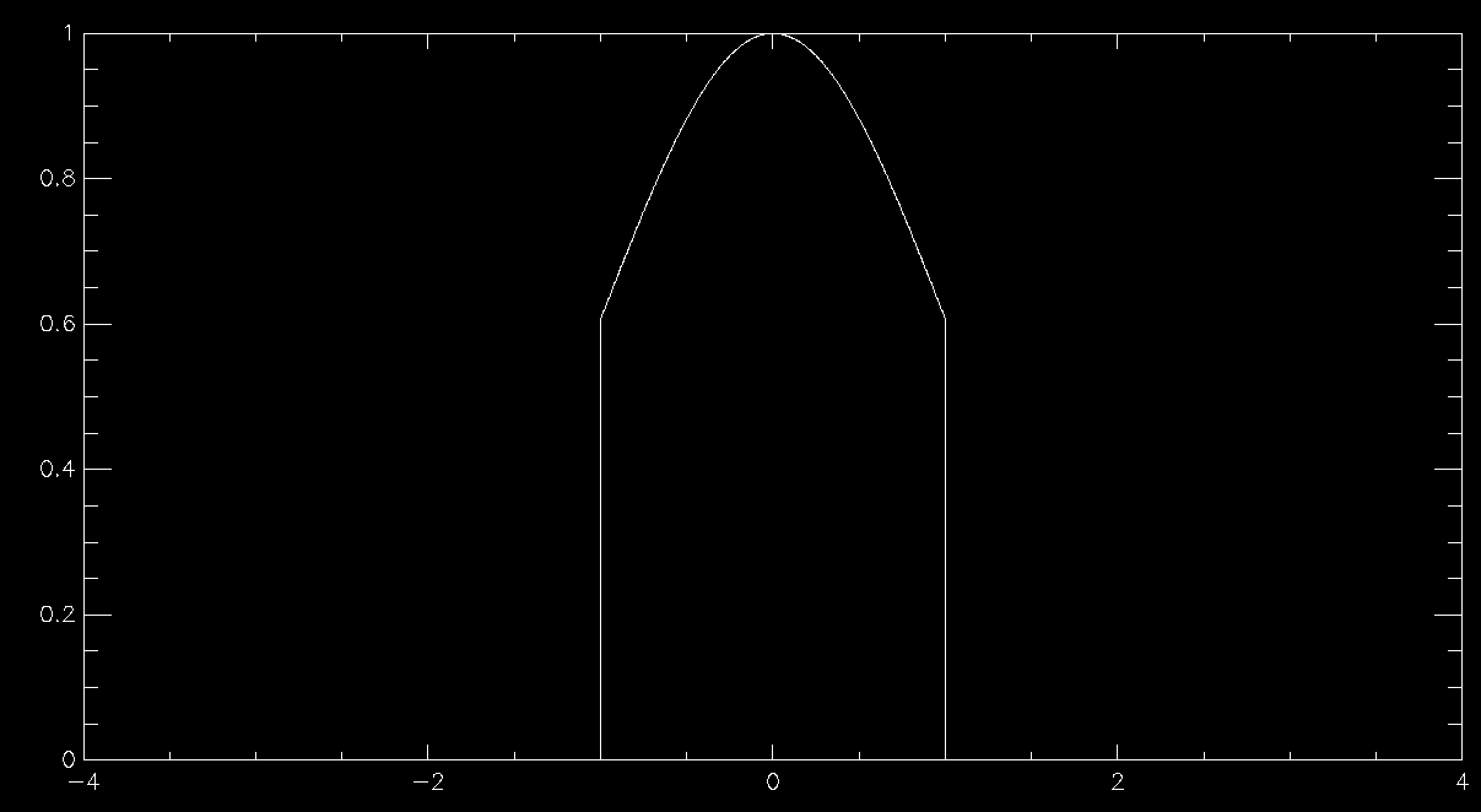
so you generally have to go further out. At 2 standard deviations you're now accepting about 60% of trials, so you're taking about 66% longer than simple sampling. At 3 standard deviations you're at 42% average acceptance and you're talking about taking 2.4 times longer than a simple sample. At 4 standard deviations you're now down at 31% average acceptance and you've having to do 3 trials for an average sample until you accept it. Unsurprisingly this takes about 3 times longer than simply being able to specify the value, but finally your Normal curve looks about right by eye. As you can see, rejection sampling really should be your last resort since Normal curves are about as benign as distribution functions get - most functions that you'd actually want to run acceptance sampling on have lower acceptance probabilities by the time that you are sampling everything that you want to.

There are more advanced algorithms that are better than rejection sampling (try looking at the Metropolis-Hastings algorithm if you want a place to start), so you're not completely out of luck if you've reached this point and rejection sampling is too slow, but things do start getting more complex from here on in.

Christopher Brady : 27 Jun 2018 17:36 |  Tags: Programming Randomness |  Comments (0) |  Close comments |  Report a problem

More randomness and a bit of non–randomness

Normally distributed random numbers

The last blog post was about getting high quality, uniformly distributed random numbers. In this post, I'm going to address the question of what to do if you want to have non uniformly distributed random numbers, that is random numbers where some are more likely than others. One of the ways that we're going to be looking at this is by looking at Probability Distribution Functions(PDF). These graphs are very like histograms, but they instead say "I have a source of random data U. For the entire source U, what is the probability that any given value is in the range x to x + dx, where dx is a finite but usually small deviation from x". In practice, what you do is you split up the range of U into a series of bins of width "dx" and then just count the number of particles in each bin and divide by the total number of particles.

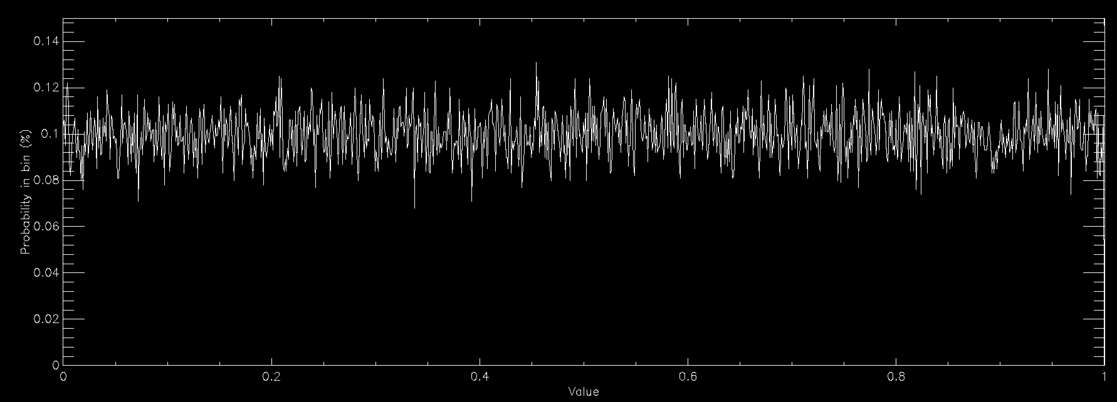
The above graph shows the probability distribution for a uniform random number when you have 1,000 bins between 0 and 1. This number of bins explains why the graph is showing a rough line centred around 0.1% probability. Since a uniform random number generator should produce values in all bins equally, you would expect (100/nbins)% (so 0.1% for 1,000 bins) to lie in each bin. The graph shows that the random number generator that I'm using is working reasonably well.

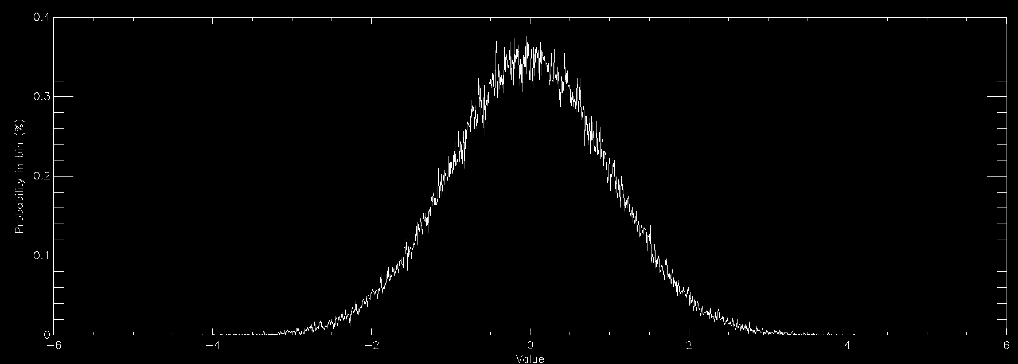
This graph shows the same thing for a normally distributed random number (also called Gaussian, or in some fields Maxwellian distributions and sometimes bell curves). It is strongly peaked at zero and extends out to ±6. Normal distributions are very important in many areas of study (see here for some examples), and is found in things as diverse as the distribution of speeds of particles in a gas to the distribution of heights of members of a sports club. As a consequence there is a lot of interest in generating normally distributed random numbers. This is often called "sampling" the distribution. The graphs above were created by getting random numbers and counting how many fell into each bin on the graph, but often you want to go the other way. You want to draw the graph and then get random numbers such that their distribution will match the graph.

Fortunately there's a very easy way of converting from a uniform random number generator to a normally distributed random number generator via an algorithm called the Box-Muller Transform. I'm not going to go into the maths of it which are detailed on the linked Wikipedia page, but if you want normally distributed random numbers the Box-Muller Transform is your friend (usually the specific variant called the Polar Box-Muller Transform). Lots of languages already have built in implementations of normally distributed random number generators, generally using that transform so it's worth looking for those first, especially in compiled languages like Python where the built in function will probably be much faster than yours. However, in languages like C or Fortran which don't have a built in one you probably want to find or write an implementation of the Box-Muller Transform if you need normally distributed random numbers.

Arbitrary distributions in one variable

Sometimes, however, you have a more complicated distribution function that you want to sample. Sometimes there are other transforms like Box-Muller, but quite often there aren't. At which point the most powerful tool you have is called Inverse Transform Sampling. This introduces a new idea the Cumulative Distribution Function (CDF). The CDF is very much like the PDF in many senses, but instead of saying "how much of U is between x and x+dx" it says "how much of U is between min(U) and x", hence the cumulative in the name. It is the accumulation of the probability of the value being at x or lower.

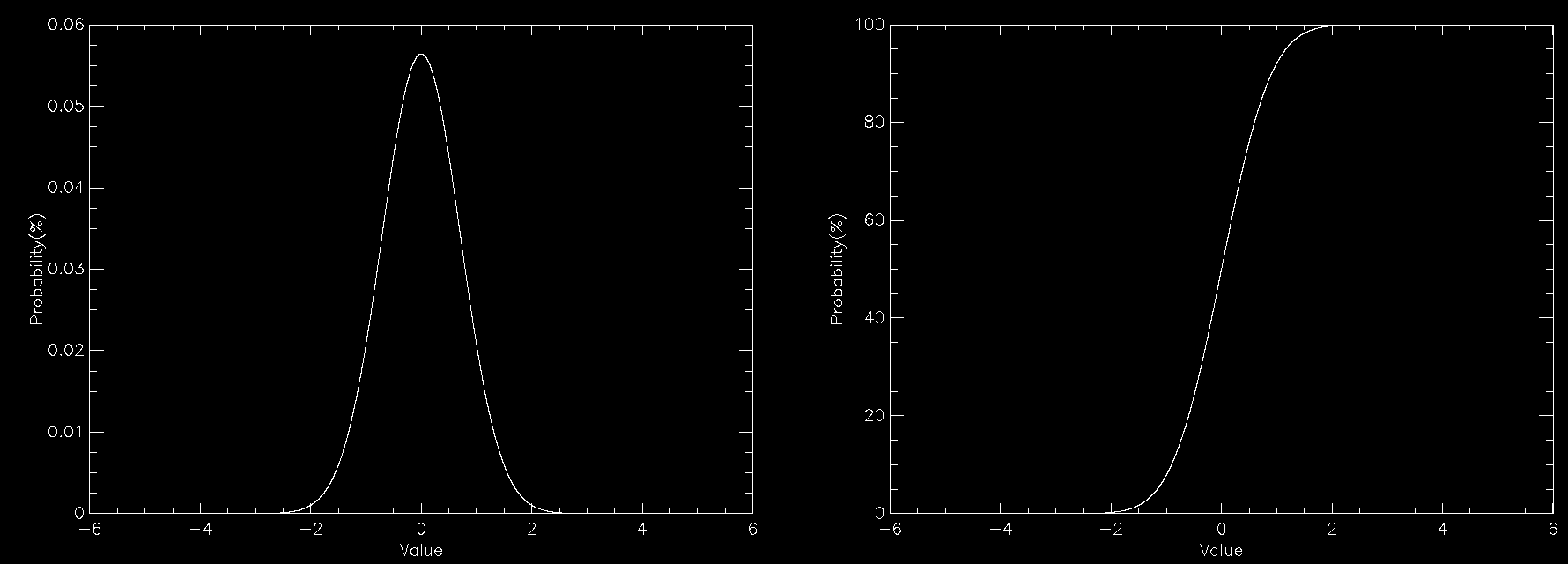
The graph this time compares the PDF (left) to the CDF (right) for a normally distributed number. The CDF has a value of 100% at the right because everything has to be less than the largest value. You can create the CDF in a number of ways, but on a computer a very common way is to define a grid of values (x(i), say) and calculate the PDF (PDF(i)) for each of them. This does mean discretising your distribution but that is often sufficient and you can often interpolate the result. The CDF is then simply defined by

CDF(i) = SUM(PDF(0:i))

where i is the index into a zero based array and is evaluated from 0 to n, where n is the number of elements in the array.

Once you have the CDF sampling it is surprisingly easy. You simply pick a uniform random number between 0 and 100 and then find out which value of i is the cell in which the CDF exceeds that value. You then have sampled the value x(i). You keep repeating this until you have sufficient values. If you then check the distribution of the values it will match the PDF that you specified. Effectively this divides the PDF into bins of equal area under the curve, and selects one bin at a time with equal probability. On the CDF graph, equal area bins correspond to a uniform division of the y axis.

The actual implementation of this can be a bit messier because while the easiest way of finding which cell of the CDF exceeds your random value is simply to start at i=0 and count up, the fastestway is to use binary bisection on the index. This works because the CDF is guaranteed to increase from left to right, so if you pick any point you know if the point that you want is to the left of that point if the value is smaller and to the right of the point if the value is larger. So you can keep dividing the space into sections until you have found the value that you want. But that is an implementation issue rather than a conceptual one.

Note also that if you can integrate the PDF to obtain a CDF, which you can then invert, you can do all of this analytically, but even simple PDFs like a Normal distribution don't have an invertible CDF.

Distributions in more than one variable

Distributions in more than one variable can be tricky. But if the function is separable, that is it can be written as two functions multiplied together, each of which is in a single variable (f(x, y) = g(x) * h(y)) each part can be sampled as above. For each complete sample you take one random sample of the function g, and one of h, and multiply them together.

Functions in more than one variable which don't break down like this are generally treated using a technique called accept-reject sampling, or some more sophisticated technique in tricky cases. More on this next time.

Christopher Brady : 31 May 2018 11:55 |  Tags: Code Programming Randomness |  Comments (0) |  Close comments |  Report a problem